Insurance
Executive TechnicalWhich factors actually caused this loss, separated from the factors that merely accompanied it, so attribution is defensible, not just plausible.
The Insurance plug-in, vocabulary, structure, and the questions your leaders ask, already mapped. Nothing here starts from a blank page.
The QuestionWhich factors actually caused this loss, not merely accompanied it?
The MethodA causal model separates confounders from causes, with counterfactual attribution computed per incident.
The AnswerA percentage-based fault apportionment defensible to a regulator, not just plausible to an adjuster.
01 The Decision
A SENIOR ADJUSTER apportions a multi-vehicle claim by constructing a causal chain: which party’s action created the conflict point, which determined severity, which eliminated the escape route. She does this for 300 claims. She knows which factors interact, which are legally material in this jurisdiction, and which are noise. A spreadsheet can store her output, the numbers that came out, but not the structure that produced them. That distinction is invisible when new claims look like old ones. It becomes visible the first time opposing counsel asks a question the formula was not built to answer.
| Capability | Spreadsheet / Rules Model | Structural Causal Model |
|---|---|---|
| Conditional relationships | Fixed weights applied uniformly | CPTs encode how each factor’s weight changes with others |
| Counterfactual answers | Re-runs formula with new input, not a counterfactual | Abduction fixes background; intervention changes one variable |
| Jurisdiction specificity | One formula or separate sheets with no structural connection | Jurisdiction-specific CPTs on a shared causal graph |
| Audit trail | Formula produces a number; no causal explanation | Every split traceable node by node through the graph |
| Novel fact patterns | Extrapolates linearly from training cases | Probabilistic inference over the causal structure; generalises correctly |
| Deposition readiness | “The adjuster used her judgment” | Point estimate with traceable causal path; auditable at deposition |
| Knowledge retention | Walks out with the adjuster | Encoded in the model; her replacement handles same complexity from day one |
02 The solution
- Given everything that was true about this specific collision, would Party B’s fault share have been different if they had been traveling at the speed limit?: Rung 3 (Counterfactual). Requires abduction to anchor the wet road, Party A’s red-light violation, Party C’s tailgating, and the jurisdiction as fixed background before changing only Party B’s speed.
- What is the causal effect of Party B’s excess speed on fault share, separated from the background conditions that made excess speed more likely in the first place?: Rung 2 (Intervention). A do(Speed = Lawful) query severs the back-door path from Jurisdiction and Road Conditions through driving behavior.
- Given that the collision was severe, what does the model infer about the most probable upstream states, speed, road conditions, visibility, and escape route?: Rung 1 (Association). The graph encodes which dependencies exist between contributing factors and collision severity.
The solution was to model the relationships between the variables that determine fault attribution, and to be explicit about which variables cause which. We recognised, for example, that visibility conditions are not independent of driver behaviour, poor visibility makes excess speed both more likely and more consequential, which means observing a high fault share tells you something about the conditions that produced it. Road surface, vehicle speed, and prior incident history all influence the outcome, but through different causal pathways: some operate through exposure, others through response capacity. When you observe a variable in this model, you are effectively filtering the data to cases where that variable takes a particular value, and that filter ripples through the model, shifting related variables up and down accordingly. When you intervene on a variable, forcing it to a value regardless of what caused it, you break that ripple effect and get a cleaner answer: not what collisions that look like this tend to produce, but what would have happened if this specific factor had been different When you abduct, you extract a particular case from the averages, locking in its idiosyncratic circumstances before asking what would have happened if one or more things had been different.
03 What the solution answers
This is the question opposing counsel asks at deposition. It requires individual counterfactual reasoning: not what happens on average when speed is lawful, but what would have happened in this specific collision. Abduct the background conditions from the factual evidence, apply do(Party B Speed = Lawful), then read the fault shares with the same U nodes held, the same collision, only B’s speed changed.
Party B’s dominant fault band shifts from 75–100% (41.0%) to 0–25% (65.7%) when their speed is made lawful. Collision Severity drops from 93.5% Severe to 58.9% Severe. Liability drops from 71.6% High to 43.4% High. Party A’s and Party C’s conduct are unchanged, A still ran the red light, C was still tailgating.
Visibility is a confounder for Party B Speed: poor visibility makes excess speed both more likely and more dangerous. When you observe lawful speed, Bayes’ theorem updates Visibility toward Clear. When you intervene with do(Speed = Lawful), the link from Visibility to Speed is severed. Visibility stays at its prior. The gap between the two queries is the confounding bias that an observational analysis cannot remove.
Under do(Speed = Lawful), Visibility stays at prior (70.0% Clear / 22.0% Reduced / 8.0% Poor). Under obs(Speed = Lawful), Visibility updates to 76.9% Clear, the back-door remains open. Any apportionment analysis that conditions on party conduct as evidence rather than intervention carries this bias. The SCM makes the distinction explicit and computable.
Diagnostic inference runs from observed effect back through the causal graph. The graph structure constrains which upstream states are inferred: speed determines severity, not fault; fault is determined by the sequence of actions that created the conflict. A flat correlation model cannot make this distinction.
Setting Collision Severity = Severe updates Party B Speed toward Reckless (44.7% up from 10.0%), Road Conditions toward Wet and Ice, and Escape Route toward Blocked (55.8% up from 38.0%). Liability shifts to 70.9% High before any party conduct is explicitly known. The model identifies B’s speed and a blocked escape route as the most likely upstream contributors, because that combination is most causally consistent with the observed severity.
04 Inside the Model
A language model can speak fluently about any domain. It cannot know one. The .bayes file is the knowledge the LLM is missing: a causal map of the domain, auditable, versioned, and wrong in specific correctable ways.
Three models, one per rung. Optionally open each in Bayes Server or any equivalent tool. The model is the thing; the software that runs it is a commodity.
A black checkmark = observed evidence. A red checkmark = do() intervention (severs incoming links; parents stay at prior).
Rung 1, Diagnostic: severity → upstream inference
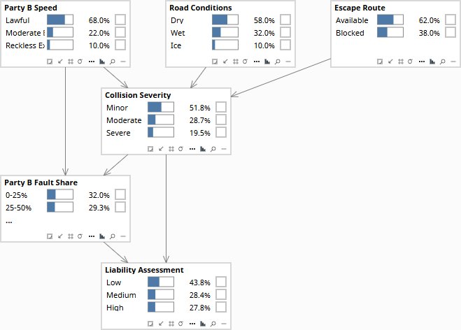
Root nodes at prior: Speed 68/22/10%, Road 58/32/10%, Escape 62/38%. Collision Severity 51.8% Minor / 19.5% Severe. Fault Share 32.0% in 0–25% band. Liability 27.8% High.
Rung 2, Intervention: do() vs obs() on speed
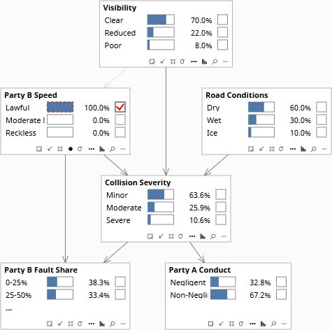
Visibility stays at prior: 70.0% Clear / 22.0% Reduced / 8.0% Poor. The back-door through Visibility is severed. Collision Severity: 63.6% Minor / 10.6% Severe. Fault Share: 38.3% in 0–25% band.
Rung 3, Counterfactual: the deposition question
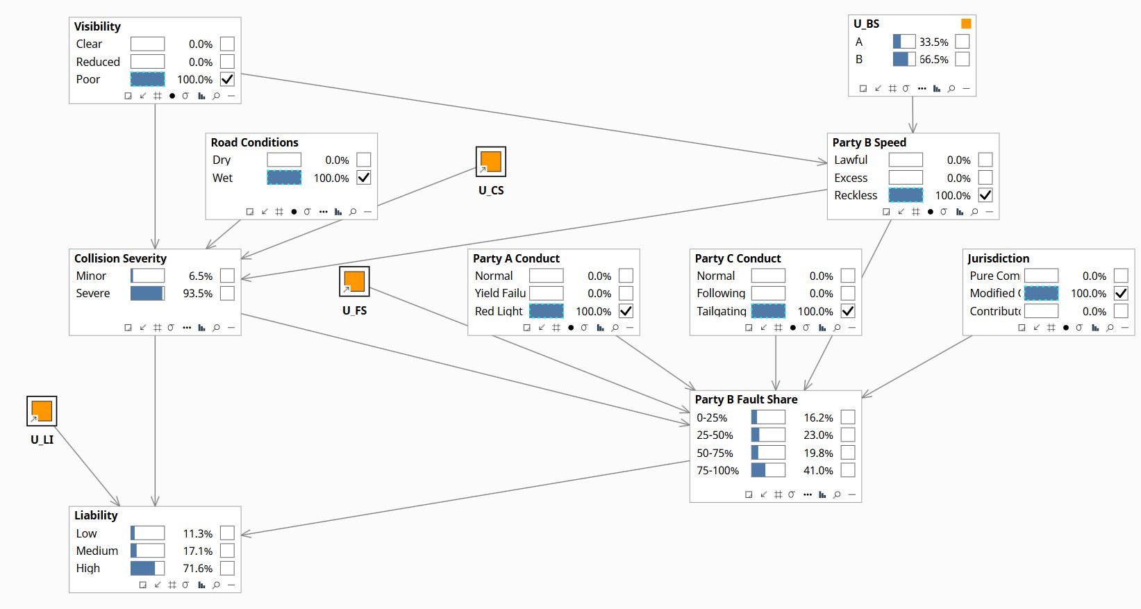
Full fact pattern entered. U_BS updates to 33.5/66.5, this collision’s driver background is anchored. Collision Severity: 93.5% Severe. Party B Fault Share: 41.0% in the 75–100% band. Liability: 71.6% High.
05 Just Ask
The model is a file. Any capable LLM can load its XML and answer apportionment questions in plain English, keeping seeing, doing, and imagining apart.
Same model, same three rungs, driven in conversation. The audit trail is the .bayes file, not the adjuster’s memory.
- Reserve adequacy. Given this fact pattern, is the current reserve too low?
- Renewal pricing. Would tightening underwriting criteria reduce losses more than raising the deductible?
- SIU referral value. If this claim had been flagged for special investigation earlier, would the payout have been lower?
- Subrogation potential. Given the fault split, what is the expected recovery from Party A’s carrier?
- Portfolio-level drift. Has the average fault attribution for this loss type shifted since the model was last calibrated?
06 The Engagement
The senior adjuster who knows how to apportion this claim is already counting down to retirement. The conversation identifies the causal structure in her reasoning, and builds the model that makes it permanent.
InsuranceAttributionSCM.bayes: Rung 3
13-node SCM with Visibility as confounder and U_BS, U_CS, U_FS, U_LI exogenous noise nodes. Three-step counterfactual: abduction anchors U nodes to the specific collision, do(Party B Speed = Lawful) severs the Visibility back-door, read Fault Share shift for this specific incident.
InsuranceAttributionIntervention.bayes: Rung 2
6-node intervention model with Visibility as confounder for Party B Speed. Compare do(Speed = Lawful), Visibility stays at prior, against obs(Speed = Lawful), Visibility updates to 76.9% Clear. The gap is the confounding bias spreadsheet apportionment cannot remove.
InsuranceAttributionDiagnostic.bayes: Rung 1
6-node diagnostic model with Party B Speed, Road Conditions, and Escape Route as root cause nodes. Enter Collision Severity = Severe; read the posterior on upstream states before any party conduct is explicitly known.
This case study is a composite drawn from multiple engagements across the insurance and liability sector. Specific figures are representative. No individual client or engagement is described. The Bayes Server models are working files: download, set evidence, and run inference.
The Deeper Trade
The model does not replace the expert who built it. It frees her from being the bottleneck for every routine version of this question, so she can spend her judgment on the cases that actually need it, and keep making the model better.