Supply Chain
Executive TechnicalWhich resilience investments would have contained last quarter’s disruption, and which ones you are buying that a confounder is making look better than they are.
The Supply Chain plug-in, vocabulary, structure, and the questions your leaders ask, already mapped. Nothing here starts from a blank page.
The QuestionWhich resilience investments would have actually contained last quarter's disruption?
The MethodA causal model separating real resilience effect from confounders inflating some investments' apparent value.
The AnswerA ranked list of which investments earn their budget, and which are riding a confounder's coattails.
01 The Decision
MOST FIRMS INVESTED IN SUPPLY-CHAIN RESILIENCE between 2018 and 2022. Buffer inventory, multi-sourcing, geographic diversification, capacity flexibility. The disruption came; some of those investments mattered, others didn’t. The honest accounting question, what did each of them buy you, and what would have happened if you hadn’t made them, has no standard answer.
The CFO question is harder than the CMO question. A CMO can ask “did this campaign produce revenue” and get measured (badly) by digital attribution. A CFO asking “did this resilience investment produce avoided loss” gets nothing, because avoided loss is structurally invisible. You can’t see the stockout that didn’t happen. You can only argue about the counterfactual.
Service level, fill rate, days-of-supply, OTIF. Useful for tracking, useless for attribution. The dashboard tells you outcomes; it doesn’t tell you which investment produced them.
“Our stockout rate was 3% during Q2 2020; competitors without buffers had 8%.” Confounded by industry segment, customer mix, supplier portfolio, geographic exposure. Same back-door problem as MMM regression.
Closest current practice gets to a counterfactual, but assumes the simulation captures all relevant dynamics. It typically misses the back-door confounders: firm-level resilience posture, market-state-dependent demand, supplier-relationship-driven access. The simulation answers a hypothetical that doesn’t quite match the world.
02 The solution
A Structural Causal Model names the latent confounders explicitly and parameterizes the analyst’s assumption about their strength. Three differences from simulation matter for a CFO conversation:
The SCM adds a ResiliencePosture latent node. The Rung-2 do-operator cuts the back-door and isolates buffer’s specific causal effect.
“What would have happened” is different from “what would happen.” The SCM’s twin-network procedure produces a firm-specific answer. Simulation produces a population expected value.
Lambda, latent-to-decision strength, latent-to-outcome strength, each is an explicit parameter. The CFO conversation becomes “this is what we conclude under these assumptions” not “trust this number.”
The structural equations (all variables standardised, disruption severity fixed at 1.5):
ResiliencePosture (R) = 0.6·M + U_R
BufferInvestment (B) = 0.5·M + 0.7·R + U_B
MultiSourcing (MS) = 0.4·M + 0.6·R + U_MS
StockoutLoss (SL) = 3.0 − 1.20·B − 0.75·MS − 0.30·R + U_SL
CarryingCost (CC) = 0.40·B + U_CC
NetBenefit (NB) = −SL − CC
True buffer net effect on NetBenefit: +0.80 per standardised unit. Naive analysis reports +0.997, a 25% overstatement from the latent confounders.
The solution was to model the relationships between the variables that drive supply chain performance, and to be explicit about which variables cause which. We recognised, for example, that resilience posture is a confounder: firms that invest more in buffer stock also tend to invest more in supplier diversification and demand sensing, which means the observed correlation between any one of those investments and disruption outcomes overstates what that investment alone would deliver. Supplier concentration and demand volatility both influence the cost of a disruption, but through different mechanisms: one determines how many alternatives exist, the other determines how quickly the situation deteriorates. When you observe a variable in this model, you are effectively filtering the data to cases where that variable takes a particular value, and that filter ripples through the model, shifting related variables up and down accordingly. When you intervene on a variable, forcing it to a value regardless of what caused it, you break that ripple effect and get a cleaner answer: not what supply chains that look like this tend to produce, but what would happen if this specific investment were made When you abduct, you extract a particular case from the averages, locking in its idiosyncratic circumstances before asking what would have happened if one or more things had been different.
03 What the solution answers
Firms with high buffer (B = +1) had NetBenefit of −1.68 vs baseline −3.00, meaning buffer inventory reduced losses but did not eliminate them. Looks valuable, but high-buffer firms are also high-posture firms, and posture independently improved outcomes.
E[NB | obs B = +1] = −1.68 (apparent benefit: +1.32)
do(B = +1) cuts buffer’s inbound arrows. Latents revert to priors. Only the direct structural effect survives. Rung-1 vs Rung-2 gap: 1.65× naive overstatement.
E[NB | do(B = +1)] = −2.20 (structural benefit: +0.80)
A specific firm observed B = +1.5 and NetBenefit = −1.2. What would NetBenefit have been if they’d set buffer to 0, holding all realised noise terms fixed? Abduct → action → predict.
E[NB* | obs(B=1.5, NB=−1.2), do(B*=0)] = −2.40
The buffer was worth +1.20 for this firm specifically. Quantitative, attribution-specific, assumption-visible.
04 Inside the Model
A language model can speak fluently about any domain. It cannot know one. The .bayes file is the knowledge the LLM is missing: a causal map of the domain, auditable, versioned, and wrong in specific correctable ways.
Optionally open ResilienceInvestment-AllRungs.bayes in Bayes Server. The model is the thing; the software that runs it is a commodity. 12-node CLG network: MarketState, ResiliencePosture, BufferInvestment, MultiSourcing, StockoutLoss, CarryingCost, NetBenefit, plus five U-noise nodes.
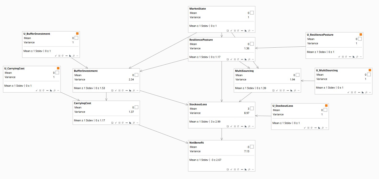
MarketState at top is the latent confounder. U-noise nodes enable Rung-3 inversion. NetBenefit marginal of −3.0 is the base disruption loss before mitigation.
Diagnostic: naive vs causal vs SCM
Buffer coefficient: +0.997 (true: +0.800, bias: +24.6%). Latents absorb into the buffer coefficient.
Buffer coefficient: +0.829 (true: +0.800, bias: +0.029), within sampling noise when latents are observable.
Rung 1: +1.32. Rung 2: +0.80. Rung 3 (B=+1.5, NB=−1.2): NB* = −2.40. The Rung-2/Rung-1 gap is the confounding bias the naive analysis inherits.
05 Just Ask
The model is a file. Any capable LLM can load its XML and answer resilience-attribution questions in plain English.
Same model, three rungs. The audit trail is the .bayes file, not the simulation.
- Investment stacking. Does combining two resilience investments compound their effect or overlap?
- Supplier concentration. Which single supplier failure would cause the most cascading disruption?
- Confounder isolation. Is this investment's apparent value actually just capacity we would have added anyway?
- Scenario planning. How would the network perform under a disruption twice the size of last quarter's?
- Renewal decision. Is this investment still earning its keep given how the network has changed?
06 The Engagement
Elicit the confounder structure from the people who know how the supply chain works. Parameterize from historical data. Deliver a defensible range, not a number to be accepted on faith, but an assumption-visible audit the CFO can challenge productively.
- Corrected resilience ROI per investment type, structural, not observational
- Firm-specific Rung-3 answer: what each investment was worth during your disruption
- Sensitivity analysis: how the conclusion moves as confounder-strength assumptions change
- The .bayes file, your SCM, openable and auditable
- A documented configurator playbook for adapting to the next disruption period
This case study uses a synthetic dataset generated from a known structural causal model. No individual client or engagement is described.
The Deeper Trade
The model does not replace the expert who built it. It frees her from being the bottleneck for every routine version of this question, so she can spend her judgment on the cases that actually need it, and keep making the model better.