How a Model Gets Built
Executive TechnicalElicitation, sparse data, integration, and the model library, the method from expert knowledge to a running causal model.
01 Beyond DAGs
DAGs are not the only language for causal structure.
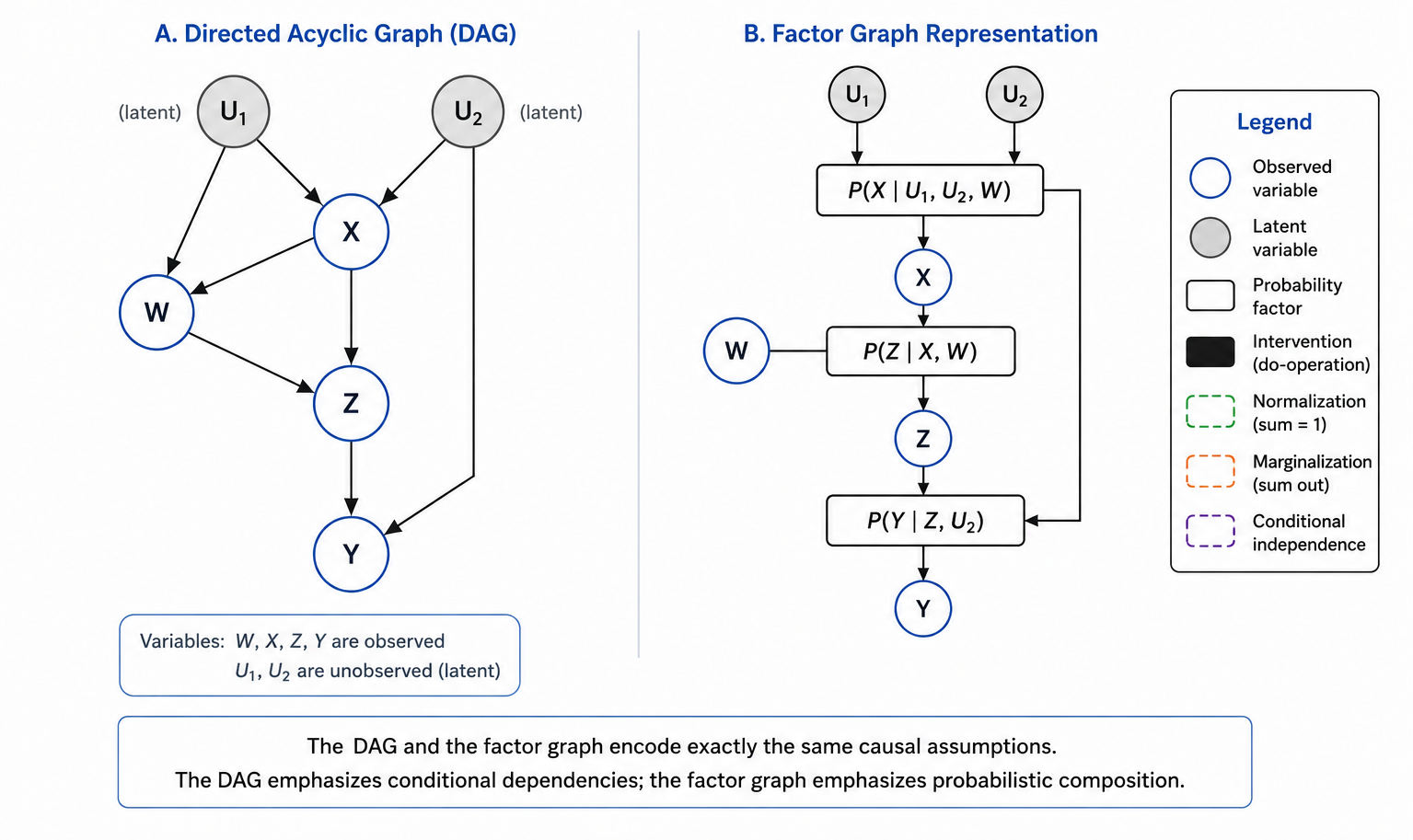
A directed acyclic graph is a powerful representation, but it is not the only one. String diagrams, from applied category theory, represent causal processes as morphisms that compose along a shared interface. Where a DAG names nodes and edges, a string diagram specifies how processes wire together and sequence. It allows algebraic reasoning across compositions without re-specifying the full graph. Recent work by Fong, Jacobs, and Zanasi has shown that several core causal inference results, including the do-calculus, can be derived cleanly in this framework, often with shorter proofs and tighter compositionality guarantees than the graph-theoretic originals.
Why Rung3 uses DAGs anyway. Enterprise causal inference tooling, Bayes Server, GeNIe, AgenaRisk, is built on the DAG / CPT / junction-tree stack. String diagrams remain a research formalism with no production implementation. The practical choice is DAGs. The intellectual horizon is wider.
02 Elicitation
Getting the model out of the expert’s head.
If the domain model can’t be learned from your data, it has to come from the people who carry it. Elicitation is the discipline of turning what a senior expert knows, often tacitly, into a graph and a set of mechanisms a machine can run. This is the hard part, and it is where most of the method lives.
It is not an interview. The expert rarely volunteers a DAG; they volunteer judgments, war stories, and rules of thumb. The work is to convert those into structure and mechanism, then check the result against cases the expert will recognize.
What a senior expert is actually doing
The expensive skill isn’t recalling facts; it’s creative abduction: positing the hidden variable that explains a pattern. “These accounts churn for a reason we don’t log.” The latent cause is named, given a place in the graph, and made queryable. Most of what separates a senior expert from a junior one is a richer set of these unobserved variables; elicitation’s job is to surface them.
When experts disagree
They will, on structure and on strength. Two experts draw different arrows (a structure disagreement); two experts agree on the arrow but not its magnitude (a strength disagreement). Neither is fatal. Structure disagreements resolve by finding the case that distinguishes the two graphs and asking which answer is right. Strength disagreements are pooled, the spread carried forward as uncertainty, not averaged away. Both have full worked treatments in the reconciliation models.
Proof, an absent arrow is an assumption
Movement 1 showed that direction isn’t in the data: arrows can’t be recovered from correlation. The corollary is decisive, whoever supplies the arrows supplies identification.
Before. X and Y share a common cause. If it’s unobserved, P(Y | do(X)) is not a function of the data, not identified.
The expert’s move. Assert the structure: “the only common cause is Z, and I can measure it”, equivalently, there is no unobserved U once we condition on Z. That assertion is an absent arrow: untestable from the data, decisive for the answer.
After. The back-door criterion is satisfied: P(Y | do(X)) = ∑z P(Y | X, Z=z) · P(Z=z). Identified.
Elicitation isn’t a softer, less rigorous input than data. It is the production of exactly these arrows, the input identification actually requires.
A model you can run is now in hand. But the expert’s mechanisms are approximate and the data to sharpen them is thin. That is the next problem.
03 Sparse Data
Substituting for the data you don’t have.
The decisions that matter most are the ones you face least often: a price move in a new segment, a once-a-decade capital call, a failure mode seen twice. The data is thin by nature, and thin data is exactly where machine learning has nothing to say. A regression needs many more rows than parameters; at a dozen records it overfits, at three it can’t start. The honest output of ML on sparse data is a shrug.
An elicited model doesn’t wait for the data to exist. The expert’s mechanism is already a full predictive distribution, a prior: so the model answers from the first day, with a calibrated error bar instead of a shrug. Then, as records arrive, you don’t retrain. You update.
Bayesian updating (averaging, but weighted by precision)
Bayesian updating fuses what you believed with what you just saw, each weighted by its precision: the inverse of its variance. A confident expert and a noisy measurement: the expert dominates. A vague prior and a clean reading: the reading dominates. Nothing is averaged blindly; every source counts for exactly its certainty.
Several noisy estimates of one latent quantity combine into a single sharper one:
μpost = ( ∑i μi / σ²i ) / ( ∑i 1 / σ²i )
The posterior is sharper than any input, combining estimates reduces variance.
Proof, the numbers
Three readings of one unknown weight, 10, 15, 17, on scales of differing quality (variances 1, 2, 3). Fuse them:
μpost = (10/1 + 15/2 + 17/3) / 1.833 = 12.64
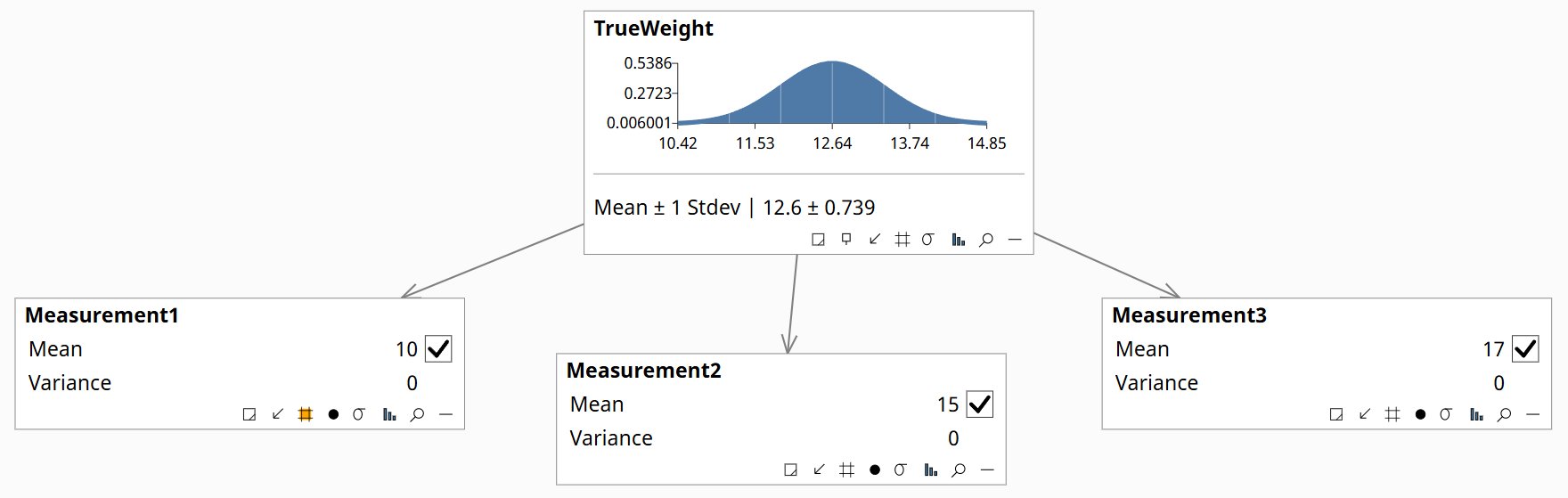
The same fusion, computed in Bayes Server.
The fused estimate is tighter than the best single scale, variance 0.545 against 1.0. Now read the first reading as an expert prior and the rest as data: the math is identical. The expert is simply the first, usually most precise, estimate; sparse data sharpens it, it doesn’t have to replace it.
The contrast is the whole point. At N = 3 a regression returns nothing usable. The Bayesian model returns 12.64 ± 0.74, an answer and an honest error bar, and tightens with every record after.
Download the worked model (.bayes) →, enter the readings one at a time and watch the posterior tighten.
This is why elicitation and sparse data are one method, not two. The expert gives you a model when you have no data; precision-weighted updating makes every scrap you later collect count for exactly what it’s worth. With a model that answers and improves, the only thing left is to let people put questions to it in plain language.
04 Integration
LLM → SCM → LLM.
The language model is the interface, not the reasoner. It reads the question, decides what is being asked, hands a precise query to the causal model, and turns the model’s answer back into language. The reasoning happens in the model; the LLM translates in and narrates out.
The LLM owns the two ends, language in, language out. The single bridge it must get right is the estimand: which probability the question is really asking for.
A worked instance, a subscription business weighing a price cut, the textbook Rung-2 decision: “If we cut price 10%, what happens to churn?” The LLM recognizes a Rung-2 question, forms the estimand P(churn | do(price↓)), compiles it to an exact inference on the SCM, and narrates the posterior back, with the error bar intact.
What runs underneath
Proof, the silent failure
The danger isn’t a wrong answer that looks wrong; it’s a wrong answer that sounds right. Ask the churn question of a language model alone and it answers fluently, from association. But the words of a question do not carry their own rung.
Question: “what happens to churn if we cut price?”
Same words, two rungs, two numbers, and the wrong one is the confident one. The integration’s whole job is to force the rung to be named: the LLM can’t tell the two apart from the words, and the model can’t be asked the wrong one without saying so.
That is the unit of work, one question, correctly routed, truthfully answered. The next step is to scale it: not one model, but a library.
05 The library
One model is a tool. A library is an asset.
A single SCM answers one domain. An organization runs on dozens of coupled decisions, pricing touches churn touches capacity touches risk. So the deliverable isn’t a model; it’s a versioned library of them, each elicited from the people who own that domain, together forming the organization’s explicit domain model. Three properties make a library more than a folder of files.
Composition
Models connect, the posterior of one is evidence for the next. A pricing model’s output feeds a churn model; a supplier-risk model feeds a capacity model. Questions cross domains without a human stitching spreadsheets together. That hand-off holds only where the shared variable d-separates the two models, otherwise the seam leaks dependence, and the join must be checked on the merged graph.
Provenance
Every arrow and every parameter carries its source: which expert, which session, which document or dataset, and when. The library is auditable: you can show a board or a regulator not just the answer but the chain of assumptions behind it. That is the difference between a model you trust and a model you can defend.
Scope & validity
Each model declares the regime where it holds. Ask a question outside that regime and the library refuses rather than fabricates, the exact opposite of a language model’s confident extrapolation past the edge of what it knows.
Proof, a composed query, and its trail
“If our tier-2 supplier’s failure rate doubles, what happens to on-time delivery?” routes through both models, the posterior of the first becomes evidence for the second. The answer arrives as a distribution and a provenance trail naming every assumption it rests on. No single dataset contains this question; the composed library answers it anyway.
A library that composes, remembers its sources, and knows its limits is no longer a consulting deliverable, it is infrastructure the organization owns and compounds. Which points at the real product: not a model, but the standing capability to keep building them.
06 The transformation
The deliverable isn’t a model. It’s an organization that reasons causally.
Everything to here describes one model and one question. The engagement leaves the organization with more than that. A library its people can read, extend, and defend. The habit of asking “what will this cause?” instead of “what does the data show?” A capability that compounds with every decision domain added. That is the transformation. It is what Rung3 advises.
The shape of the work
The engagement is Movements 3 through 7, run on one decision domain at a time: elicit the experts, stand up the model, fuse what data exists, wire it to the LLM, fold it into the library. Eight to sixteen weeks per domain. The first leaves you with a working model and a team that can run it; each one after is faster, because the method and the library are already in place.
What that capability looks like in full, one domain, every rung, composed and mediated, is the movement that follows.
07 Healthcare, In Full
Healthcare: one library, mediated.
The whole method, on one domain, what Movements 3 through 7 produce: the working artifact an organization is left with, a clinical library it reasons with across all three rungs, put to it in plain language.
One model, all three rungs
Start with a single elicited model, a patient’s medication burden and its effect on weight, cholesterol, hospitalisation, and mortality. The same model answers a different question at each rung:
Step through the model answering each in turn:
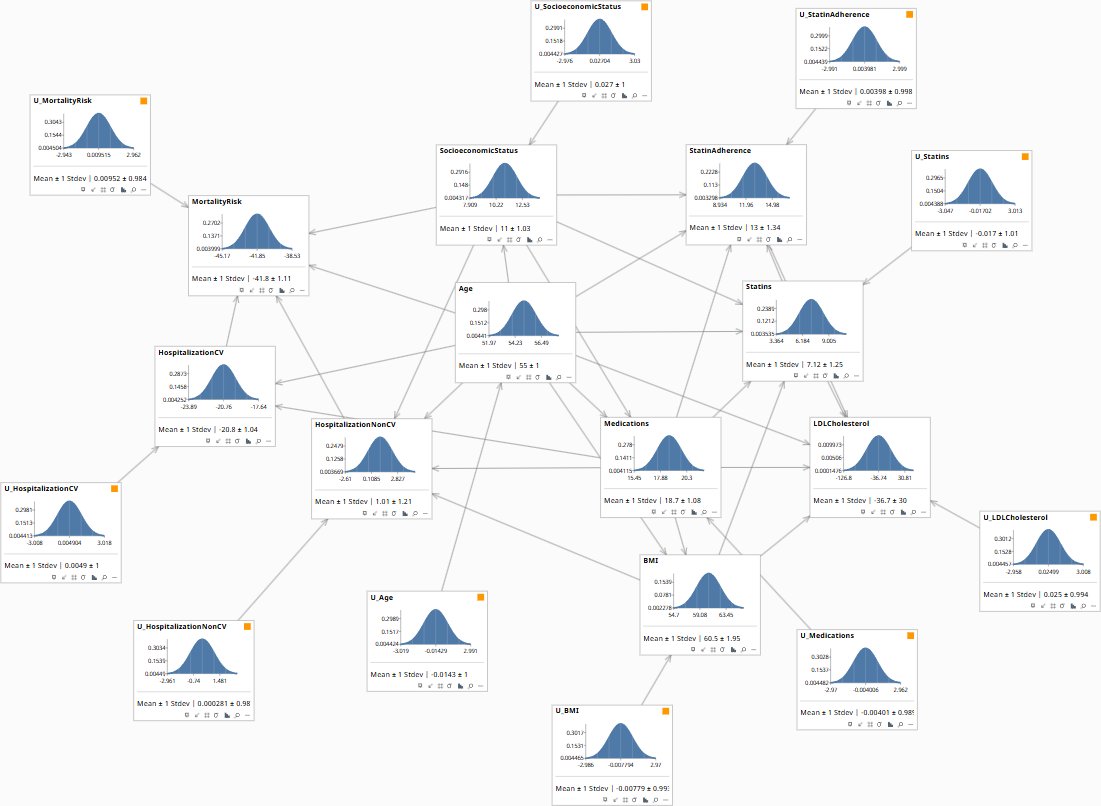
Same model, three rungs. The data never changed, the question did, and only a structural model tells the three apart. The organization gets exactly this for every clinical sub-domain it stands up.
Many models, one library
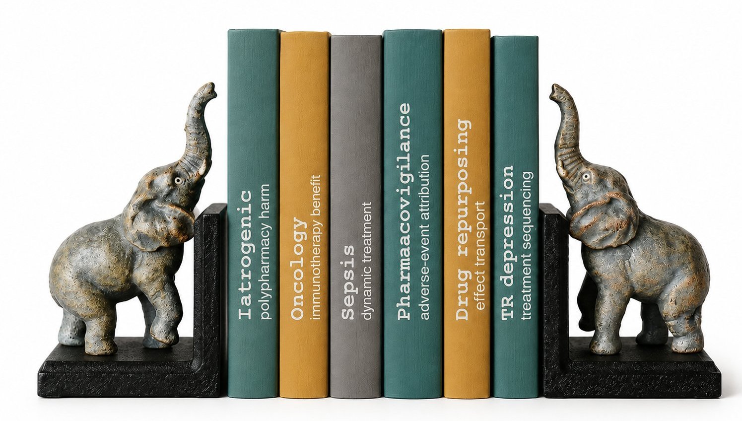
Each sub-domain is its own elicited SCM, scoped to the decisions it was built for. They are not siloed files: they share variables, and a posterior computed in one becomes evidence in the next, so a question can cross domains without a person stitching spreadsheets together. That hand-off is sound only when the shared interface d-separates the two modules, a condition checked on the merged graph and recorded in each model’s scope, so a composition carries its own license.
They converge on one composed clinical model, a cardiometabolic domain model linking blood pressure, cholesterol, diabetes, and heart disease to hospitalisation, mortality, and cost. Every node carries its provenance; each model declares its regime, so a query outside scope returns bounds or a refusal rather than a fabricated point.
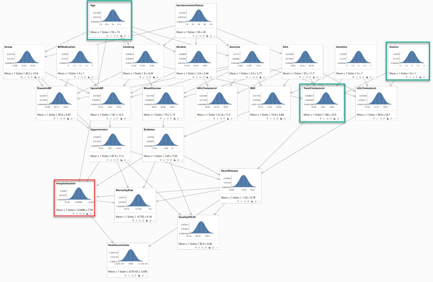
The composed clinical model. Intervention levers (age band, statins, cholesterol) feed the cardiometabolic chain; hospitalisation, mortality, and cost sit downstream. Each sub-domain model above plugs into this surface.
“If she starts immunotherapy, how does the added cardiotoxicity change her ten-year cardiac outlook?” routes through two models: the oncology SCM returns a toxicity posterior, which becomes evidence in the cardiometabolic model. The answer carries both effects and the trail of assumptions behind them, a question no single dataset contains.
Mediated by an LLM
The clinician never names a model or a rung. The language model reads the question, routes it to the right sub-model and the right rung, runs the exact query, and narrates the posterior back, the loop from Movement 5, now over the whole library. Two exchanges, two routes.
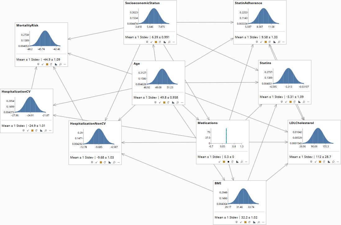
do(Medications): the node is clamped (the spike), its inbound edges severed; the downstream monitors settle to their post-intervention posteriors.
What the LLM answers alone: the population guideline, the deprescribing rule, the trial’s average survival, fluent and confident. The words of a question carry neither their rung nor their model; the library supplies both.
Worked example: sepsis, LLM-mediated →
The models
Every model in the library ships as a runnable file, authored in Bayes Server for the examples here, queried from R or Python, yours to keep. Bayes Server and its peers are about as “No Code” as we can get.
The same method runs across insurance, finance, marketing mix, and policy, the engagements →
The wedge from Movement 1 holds all the way down. You cannot learn a domain model of your business from your business’s data, but you can elicit it, run it, and compound it. That is the capability Rung3 builds, and it is the one that doesn’t leave when the engagement ends.
Most of the funded causal-AI field tries to mine cause and effect from a company’s own data. This method does the opposite. Here’s the full map of who’s selling what, and the corner Rung3 holds alone.
08 Where It Sits
Each section of this page has a dedicated page in the Architecture series, where the mechanism is described in full detail with worked examples, schemas, and LLM dialogues.