Foundations
TechnicalEARA is not adjacent to data science and AI. It is a specific architectural pattern for deploying causal inference, Bayesian reasoning, and neurosymbolic AI in enterprise production. These are the intellectual foundations it builds on.
01 Pearl’s Ladder
The organising framework. Three rungs. Everything else follows from them.
The three rungs of causation, association, intervention, counterfactual, are the organising framework of modern causal inference in statistics and data science. Pearl’s do-calculus, the backdoor criterion, and the frontdoor criterion are standard tools in observational study design. They determine whether a causal quantity is identifiable from observational data, and if so, how to estimate it.
EARA operationalises these as a runtime architecture rather than a methodological framework. The Pipeline routes each incoming query to the correct rung before running inference. The rung is a first-class dimension of every query, not an afterthought. Rung 1 queries run belief propagation. Rung 2 queries invoke the do-operator and sever the incoming edges to the intervention variable. Rung 3 queries run the abduction-action-prediction procedure on the structural causal model with U-nodes.
What EARA adds to the literature. Pearl’s framework specifies what can be computed and under what conditions. EARA specifies how to build a production system that computes it, with a language interface, a certificate, an audit trail, and a monitoring layer that detects when the model is no longer a good description of reality.
Pearl, J. & Mackenzie, D. (2018). The Book of Why. Basic Books. · Pearl, J. (2009). Causality (2nd ed.). Cambridge University Press.
02 Bayesian Networks
The engine is mainstream. The discipline behind it is not.
In this practice, a causal model is a Bayesian network. The terms are used interchangeably throughout the site.
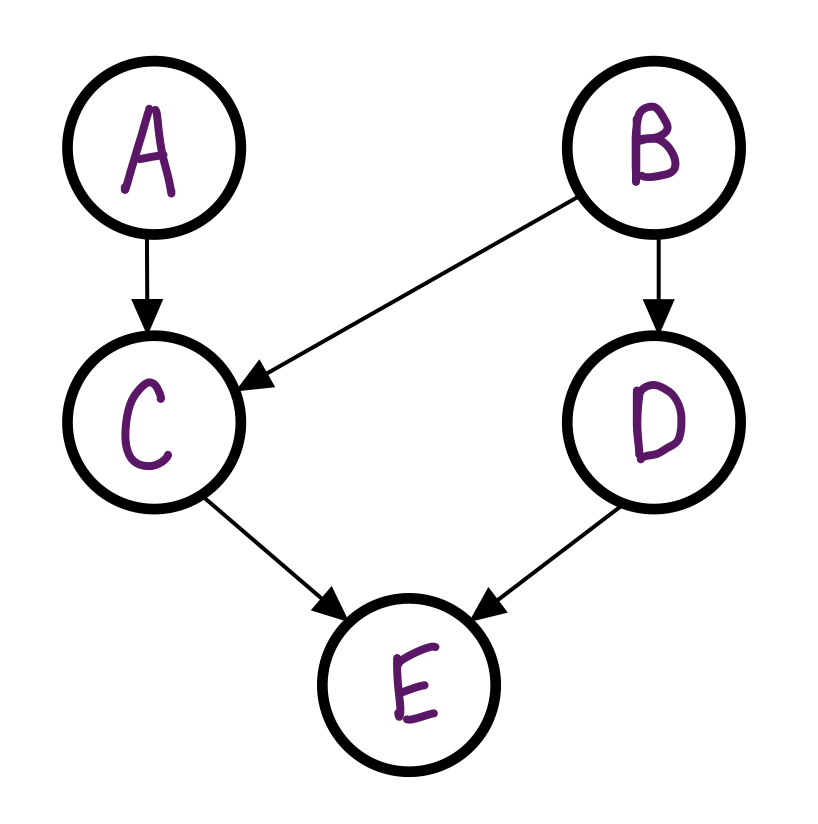
A Bayesian network is a directed acyclic graph (DAG) in which each node represents a variable and each edge represents a direct causal or probabilistic influence. The graph encodes which variables affect which others; the conditional probability tables at each node encode how strongly. Together, graph and tables define a joint probability distribution over all variables in the model.
Given observed evidence, a sensor reading, a clinical result, an analyst’s judgment, the network propagates that evidence through the graph and updates every connected variable’s probability. That propagation is Bayesian updating: the belief state of the whole network revises in response to each new observation, weighted by how informative the observation is.
Bayesian networks are a mainstream tool in machine learning and decision analysis. They are used in medical diagnosis, fraud detection, fault diagnosis, predictive maintenance, and risk assessment across insurance, energy, and cybersecurity. The junction tree algorithm, belief propagation, and conditional linear Gaussian distributions are standard computational statistics.
Bayes Server, the engine behind this practice, implements the same probabilistic graphical models used in production across aerospace, defence, energy, pharmaceuticals, and national governments. It is named in Gartner’s Hype Cycle for AI.
What makes this practice different. In most applications of Bayesian networks, the graph is learned from data or specified by a statistician as a modelling assumption. In this practice, the graph is elicited from domain experts, the people who understand the mechanisms, not just the correlations. The data inform the parameters within the structure; they do not determine the structure. This is a deliberate design choice that makes the model auditable, extensible, and transferable.
Koller, D. & Friedman, N. (2009). Probabilistic Graphical Models. MIT Press. · Jensen, F.V. & Nielsen, T.D. (2007). Bayesian Networks and Decision Graphs. Springer.
03 Structural Causal Models
The but-for test, made computable.
The structural causal model formalism, a DAG plus structural equations plus exogenous noise terms, is the same framework used in econometrics, psychometrics, and epidemiology for decades. Structural equation models are used to separate direct and indirect effects, identify confounders, and estimate causal effects from observational data.
The key difference in this practice: SCMs are used for runtime inference, not parameter estimation from observational data. The structural equations encode the expert’s model of the mechanism. The exogenous U-nodes encode the background heterogeneity that makes counterfactuals case-specific rather than population-average. The Balke–Pearl response-function encoding handles discrete variables; CLG models handle continuous ones.
The but-for test. Every counterfactual in the case study pages, whether in litigation, clinical decision support, or post-mortem attribution, is computed by the same three-step procedure: abduction (anchor U-nodes to the observed case), action (intervene on the counterfactual variable), prediction (read the outcome). This is the formal definition of the but-for test used in legal causation, translated into a computable operation on a structural causal model.
Pearl, J. (2009). Causality, ch. 7. · Balke, A. & Pearl, J. (1994). Counterfactual probabilities. UAI 1994.
04 Neurosymbolic AI
Neural networks handle language. Causal models handle cognition. EARA routes between them.
LLM + causal model is a specific instance of the neurosymbolic AI research agenda, combining neural networks (subsymbolic, learned from data, fluent with language) with symbolic reasoning systems (explicit, structured, auditable, causally grounded). This is an active research area at MIT, IBM, DeepMind, and in Pearl’s own group.
The dual-process reading is precise. Rung 1 operations, association, pattern recognition, prediction, are what neural networks do well. Rungs 2 and 3, intervention and counterfactual, require explicit causal structure that neural networks do not encode and cannot compute. The LLM handles language at both ends. The causal model handles cognition.
EARA as a neurosymbolic reference architecture. Most neurosymbolic AI research is at the model level, how to train a system that combines neural and symbolic components. EARA is at the systems level, how to build a production architecture that routes queries to the right component, certifies the output, and audits the reasoning. It is an engineering specification, not a training procedure.
Marcus, G. & Davis, E. (2019). Rebooting AI. Pantheon. · LeCun, Y. (2022). A Path Towards Autonomous Machine Intelligence. OpenReview. · Mao, J. et al. (2019). The Neuro-Symbolic Concept Learner. ICLR 2019.
05 Counterfactual ML
Would the decision have been different? That is a Rung 3 question, and only a structural model can answer it.
The counterfactual reasoning at Rung 3 directly overlaps with the counterfactual fairness literature in machine learning. Counterfactual fairness asks: would this decision have been different if a protected attribute had been different, holding everything else constant? This is precisely the but-for question, the same estimand computed in CASE2-Litigation and in the clinical counterfactuals in CASE2-Healthcare.
The Individual Treatment Effect (ITE), what would have happened to this specific person under the alternative treatment, is a Rung 3 quantity. Population-average treatment effects (ATE, ATT, ATU) are Rung 2 quantities estimable from observational data under the appropriate identification conditions. The distinction matters: a regulator asking about this specific applicant needs a Rung 3 answer; a policy-maker asking about the population needs a Rung 2 answer.
The identification problem. Rung 3 quantities are not identifiable from observational data alone without additional structural assumptions, specifically, the functional form of the structural equations and the distribution of the U-nodes. This is not a limitation unique to this practice; it is a fundamental result in causal inference. The structural causal model makes these assumptions explicit and auditable, which is precisely what makes the counterfactual defensible in a legal or regulatory context.
Kusner, M. et al. (2017). Counterfactual Fairness. NeurIPS 2017. · Hälvä, I. et al. (2021). Desiderata for Representation Learning. arXiv:2106.08340.
06 Explainability
Post-hoc explanation approximates. Structural explanation is the computation.
The auditability argument in Against Black Boxes overlaps with the LIME, SHAP, and interpretable ML literature, but with a fundamental difference that the site makes explicit. Post-hoc explanation methods approximate a black box’s behaviour after the fact. A causal model’s explanation is structural: the certificate is produced by the same computation that produced the answer.
Gary Marcus’s critique of deep learning is directly relevant. A system that encodes knowledge implicitly, in weights adjusted by gradient descent, cannot be wrong in a specific, correctable way. It can only be retrained. A structural causal model is wrong in specific, locatable ways: a specific edge that should not be there, a parameter that is miscalibrated, a confound that was not encoded. The fix is also locatable.
Faithfulness vs approximation. SHAP values are defined as the Shapley values of a model’s prediction function, a game-theoretic attribution of the output to input features. They measure sensitivity, not causation. A high SHAP value for a feature means the model’s output is sensitive to that feature, not that the feature caused the outcome. The causal model produces a different kind of attribution: which variables in the structural equations actually drove the posterior, and by how much. These are different numbers with different interpretations.
Ribeiro, M.T. et al. (2016). "Why Should I Trust You?" LIME. KDD 2016. · Lundberg, S. & Lee, S.I. (2017). A Unified Approach to SHAP. NeurIPS 2017. · Marcus, G. (2018). Deep Learning: A Critical Appraisal. arXiv:1801.00631.