Why a Causal Model
Asset reliability management has a fundamental measurement problem: the successes are invisible. A predictive maintenance program that detects a developing fault and triggers early intervention prevents a failure that never appears in the data. The board sees the cost of the program and the count of failures that occurred. It cannot see the failures that did not occur. Standard practice — comparing failure counts before and after, or against a benchmark fleet — contains a structural error: the fleets that adopt predictive maintenance tend to be higher-risk fleets, so any comparison conflates the effect of the program with the background risk that motivated the investment in the first place.
The same problem appears in interval decisions. When a board observes that fleets running extended overhaul intervals have higher failure rates, it is seeing two effects: the interval extension itself, and the elevated wear rates that tend to accompany the cost pressures that produce interval extensions. Separating those two effects requires a causal model that holds the confounder — fleet utilization pressure — at its natural level while forcing the interval to change.
| Analysis Component | Standard Approach | Causal Approach |
|---|---|---|
| Program evaluation | Count failures that occurred | Estimate failures that would have occurred without the program |
| Interval extension effect | Correlated with failure rate (confounded by utilization pressure) | Isolated via do() — utilization pressure held at prior |
| Root cause of rising outage rate | Each team cites their metric | Posterior distribution over causes given the full evidence pattern |
| PdM selection bias | Not in model — high-risk fleets compared to low-risk benchmarks | Asset Risk Profile as explicit confounder |
| Counterfactual failures prevented | Not computable | Estimated from U-node-anchored individual-level model |
The Questions
- We spent $8M on a predictive maintenance program and still had three unplanned outages — would those outages have occurred without the program? — Rung 3 (Counterfactual). Answering it requires abduction to anchor this specific fleet’s background failure risk via U nodes before removing the PdM program; without U node anchoring the counterfactual reflects a population average fleet, not this one.
- If we extend gas turbine overhaul intervals from 24 to 36 months to reduce capex, what does that actually cause to the probability of failure before the next planned intervention? — Rung 2 (Intervention). A do() query severs the confounding path from Fleet Utilization Pressure through the interval decision, isolating the causal effect of the extension from the operational environment that tends to drive both utilization and maintenance deferrals simultaneously.
- Our forced outage rate has risen 18% over three years — engineering says fleet aging, operations says increased load, finance says deferred maintenance. What does the asset data actually support? — Rung 1 (Association). The graph encodes which dependencies exist between Asset Age, Load Factor, Maintenance Spend, and outage outcomes; entering the observed trend updates every genuinely connected upstream node, separating what the data supports from what each team is asserting.
Reading the screenshots: a black check mark on a node means it has been set as observed evidence — a fact entered into the model, acting as a filter. A red check mark means it has been set as a do intervention — a decision applied to the model, severing the influence of its parents.
Reading the spec tables: each Run the Analysis block lists the exact steps to reproduce each screenshot in Bayes Server. The Obs / Do column uses three italic control tokens: clear — reset the model to a blank no-evidence state; abduction step — enter the factual observations that anchor the U nodes to this specific case; use abduction result — apply a do() intervention with the U nodes held from the abduction step.
Did the program prevent failures we cannot see?
“We spent $8M on a predictive maintenance program last year. We still had three unplanned outages. Would those outages have occurred without the program — or did it actually prevent worse failures that never appear in the data?”
This question conditions on what actually happened — three outages with PdM running — and asks what would have occurred in a world where the program had not been deployed. It cannot be answered by comparing this fleet to a non-PdM benchmark, because fleets that invest in predictive maintenance tend to be higher-risk fleets. The Asset Risk Profile confounder in the model captures this: high-risk fleets adopt PdM precisely because they fail more, so any naive comparison overstates the program's benefit. The model separates those two effects.
The U nodes (shown in orange) represent the unobserved background of this specific fleet — sensor placement quality, analyst expertise, the particular fault modes present this year, crew positioning when failures occurred. By entering the three observed outages as evidence, the model infers what those background factors must have been for this fleet in this year. It then holds those background factors fixed and asks: with everything else about this fleet unchanged, what would the failure count have been without the program?
The counterfactual comparison shows that removing PdM from this fleet's actual background has negligible effect on Outage Consequence — but that is because the U nodes are also anchored to the observed failure state. Step 2 (obs PdM=Not Implemented + Failure=Three to four) anchors the model: EFDR drops to 63.9% Low, Asset Risk shifts only modestly (28.8/55.4/15.8%), and Outage Consequence shifts to 38.5% Severe / 17.0% Contained. Step 3 shows the fleet without PdM evidence but holding the same failure event: EFDR rises to 47.7% Low vs 63.9% — confirming that the program's direct causal contribution to detection is real. Step 4, do(PdM=Implemented), severs the Asset Risk back-door: Asset Risk jumps to 47.4% High-risk (the model now correctly infers this is a high-risk fleet — only such fleets adopt PdM), EFDR improves to 46.5% High, and the failure distribution returns close to prior (24.3/34.8/30.2/10.7%). The core counterfactual insight: without PdM, this fleet's EFDR falls to 63.9% Low, which is the pathway through which unplanned failures compound.
| Image | Obs / Do | Node | Set | Result |
|---|---|---|---|---|
| ar-c-1-prior | — | PdM Program | 36.4% Implemented / 63.6% Not Implemented | |
| — | Early Fault Detection Rate | 22.6% High / 31.4% Moderate / 45.9% Low | ||
| — | Unplanned Failure Events | 24.7% Five+ / 35.1% Three-four / 29.8% One-two / 10.4% None | ||
| — | Outage Consequence | 35.3% Severe / 37.0% Moderate / 27.7% Contained | ||
| ar-c-2 | obs | PdM Program | Not Implemented | |
| obs | Unplanned Failure Events | Three to four | Abduction — fleet background anchored | |
| — | Asset Risk Profile | 28.8% High / 55.4% Moderate / 15.8% Low | ||
| — | Early Fault Detection Rate | 7.5% High / 28.7% Moderate / 63.9% Low | ||
| — | Outage Consequence | 38.5% Severe / 44.5% Moderate / 17.0% Contained | ||
| ar-c-3 | obs | Unplanned Failure Events | Three to four | Failure only — PdM not set (compare to step 2) |
| — | Asset Risk Profile | 30.5% High / 54.0% Moderate / 15.5% Low | ||
| — | Early Fault Detection Rate | 20.2% High / 32.1% Moderate / 47.7% Low | ||
| — | Outage Consequence | 38.5% Severe / 44.5% Moderate / 17.0% Contained | ||
| ar-c-4 | do | PdM Program | Implemented | Severs Asset Risk back-door |
| — | Asset Risk Profile | 47.4% High — correct inference: only high-risk fleets adopt PdM | ||
| — | Early Fault Detection Rate | 46.5% High / 36.5% Moderate / 17.0% Low | ||
| — | Unplanned Failure Events | 24.3% Five+ / 34.8% Three-four / 30.2% One-two / 10.7% None | ||
| — | Outage Consequence | 35.0% Severe / 37.0% Moderate / 28.0% Contained |
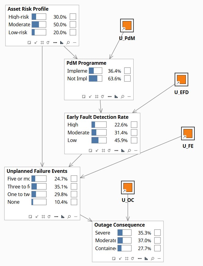
Fleet-level baseline. PdM 36.4% Implemented / 63.6% Not Implemented. EFDR 45.9% Low / 22.6% High. Failure Events: 24.7% Five+ / 35.1% Three-four. Outage Consequence 35.3% Severe.
What does extending the overhaul interval actually cause?
“If we extend the overhaul interval on our gas turbines from 24 to 36 months to reduce capex, what does that actually do to the probability of failure before the next planned intervention?”
When a board observes that fleets running extended intervals have higher failure rates, it is seeing two effects at once. Fleet Utilization Pressure independently causes both the decision to extend the interval and the wear rate on the assets — fleets under cost pressure run harder and maintain less. Observing an extended interval tells the model that utilization pressure is probably high, which raises wear rate, which worsens component condition. Forcing the interval to extended via intervention holds utilization pressure at its natural level and asks only what the longer gap between overhauls causes, separate from the operating environment that tends to accompany that decision. The gap between those two numbers is what the board needs before it approves the deferral.
do(Overhaul = Extended) raises High failure probability from 34.6% to 49.1% — a 14.5-point increase from the interval decision alone, with Fleet Utilization Pressure held at its prior. obs(Overhaul = Extended) produces 51.8% High failure — the 2.7-point gap above do() is the confounding bias: observing an extended interval updates FUP toward High (58.6% vs 30.0% prior), which further elevates wear rate and component condition. Add obs(Operating Environment = Severe) to the do() and failure probability rises to 53.4% High — the environment interaction adds another 4.3 points on top of the interval causal effect. Unplanned Outage Major rises from 33.8% at prior to 43.0% under do(Extended) alone and 45.5% under do(Extended) + Severe. The board is not deciding whether to extend the interval in the abstract — it is deciding whether to extend it on assets already exposed to severe conditions, where the effects compound.
| Image | Obs / Do | Node | Set | Result |
|---|---|---|---|---|
| ar-i-1-prior | — | Fleet Utilization Pressure | 30.0% High / 45.0% Moderate / 25.0% Low | |
| — | Overhaul Interval | 28.1% Extended / 50.4% Standard / 21.5% Accelerated | ||
| — | Component Condition | 31.6% Degraded / 36.8% Fair / 31.6% Good | ||
| — | Failure Probability | 34.6% High / 33.3% Moderate / 32.1% Low | ||
| — | Unplanned Outage | 33.8% Major / 31.0% Partial / 35.2% Avoided | ||
| — | SAIDI Contribution | 32.2% Above / 28.2% Near / 39.5% Within | ||
| ar-i-3 | do | Overhaul Interval | Extended | FUP stays at prior — back-door severed |
| — | Fleet Utilization Pressure | 30.0% High / 45.0% Moderate / 25.0% Low — unchanged | ||
| — | Component Condition | 54.8% Degraded / 31.9% Fair / 13.2% Good | ||
| — | Failure Probability | 49.1% High / 31.3% Moderate / 19.6% Low | ||
| — | Unplanned Outage | 43.0% Major / 30.6% Partial / 26.4% Avoided | ||
| — | SAIDI Contribution | 38.5% Above / 28.4% Near / 33.2% Within | ||
| ar-i-4 | obs | Overhaul Interval | Extended | Compare to do() — back-door open |
| — | Fleet Utilization Pressure | 58.6% High — up from 30.0%; confound flows back | ||
| — | Component Condition | 59.9% Degraded — higher than do() | ||
| — | Failure Probability | 51.8% High — 2.7pp above do(); confounding bias | ||
| — | Unplanned Outage | 44.5% Major / 25.1% Avoided | ||
| ar-i-2 | do | Overhaul Interval | Extended | + environment stress |
| obs | Operating Environment | Severe | ||
| — | Wear Rate | 49.1% Accelerated — environment drives wear | ||
| — | Failure Probability | 53.4% High — 4.3pp above do() alone | ||
| — | Unplanned Outage | 45.5% Major / 24.3% Avoided | ||
| — | SAIDI Contribution | 40.1% Above Threshold |
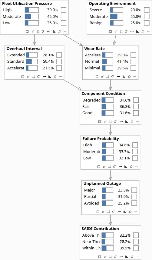
Fleet baseline. FUP 30% High / 45% Moderate. Overhaul 28.1% Extended / 50.4% Standard. Failure Probability 34.6% High / 32.1% Low. Outage 33.8% Major / 35.2% Avoided. SAIDI 32.2% Above Threshold.
Which team is right about the rising outage rate?
“Our forced outage rate has risen 18% over three years. Engineering says it’s fleet aging. Operations says it’s increased load. Finance says it’s deferred maintenance. What does the asset data actually support?”
At Rung 1 the model runs as a filter: enter what the data shows, read which root causes become more probable. Two confounders in the graph make the diagnostic discriminate between the three teams rather than updating each cause proportionally. Asset Program Maturity independently drives both Fleet Age Profile and Maintenance Deferrals — confirming Significant deferrals updates program maturity, which also shifts fleet age beliefs. Grid Demand Growth independently drives both Load Stress and Fleet Age Profile — confirming Above Rating load updates demand growth, which shifts fleet age beliefs through a different mechanism. Each team's evidence produces a different footprint across the graph, and those footprints tell the board whose hypothesis most fits the full pattern of evidence when all three data points are available.
The elevated outage rate alone cannot name a single cause — but the three teams' evidence produces meaningfully different diagnostic signatures, and the combination points most strongly to fleet aging amplified by demand growth. With only the elevated outage rate entered, all three root causes update modestly upward and no team's hypothesis dominates. Confirming Above Rating load pulls Grid Demand Growth sharply upward, which also shifts Fleet Age Profile — the operations team's evidence implicates engineering's cause through the shared confounder. Confirming Significant maintenance deferrals pulls Asset Program Maturity toward Mature, which shifts both Fleet Age and Deferrals upward — finance's evidence implicates engineering through a different route. The model does not resolve the debate; it shows that all three teams are describing the same underlying pressure through different observational windows, and that the right intervention is at the confounder level — program renewal and load growth management — rather than addressing any single symptom in isolation.
| Image | Obs / Do | Node | Set | Result |
|---|---|---|---|---|
| ar-d-1-prior | — | Forced Outage Rate | — | |
| — | Financial Impact | — | ||
| ar-d-2-elevated | obs | Forced Outage Rate | Elevated | |
| — | Fleet Age Profile | — | ||
| — | Load Stress | — | ||
| — | Maintenance Deferrals | — | ||
| ar-d-3-load | obs | Forced Outage Rate | Elevated | |
| obs | Load Stress | Above Rating | ||
| — | Grid Demand Growth | — | ||
| — | Fleet Age Profile | — | ||
| ar-d-4-deferrals | obs | Forced Outage Rate | Elevated | |
| obs | Maintenance Deferrals | Significant | ||
| — | Asset Program Maturity | — | ||
| — | Fleet Age Profile | — |
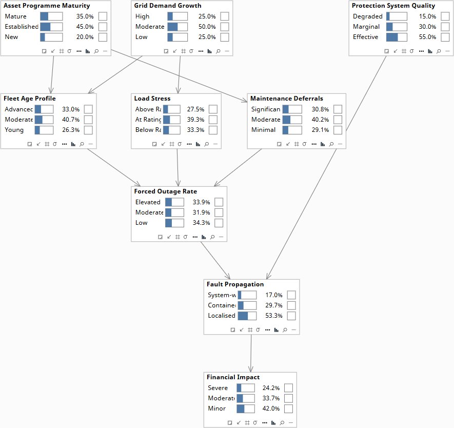
Root causes at fleet prior. Forced Outage Rate, Fleet Age, Load Stress, and Maintenance Deferrals at their baseline marginals.
Download the Models
All models require Bayes Server (free edition available). See Download Models for the full library across all case studies.
Your reliability engineers know which assets are symptomatic and which programs are under pressure. That knowledge needs to be in a causal model before the next capital allocation cycle — not discovered after the overhaul deferral produces a forced outage at peak demand.
The models are free. What I provide is the judgment to build the right structure for your specific fleet, encode your engineers’ knowledge into it, and turn the output into decisions your board can act on. The discipline stays with your team.