The three variables: Education (on a scale where 0 means no postgraduate degree and 1 means a PhD, following Pearl & Mackenzie’s coding), Experience (years on the job), and Salary (US dollars). The example is illustrative, not a fit to any particular dataset; the parameters are chosen to make the structural moves visible at each rung.
Rung 1 — Seeing
The first rung is what data and statistics can do unaided: observe joint distributions, condition on observations, report what tends to occur with what. The structural question — which variable causes which — is out of scope.
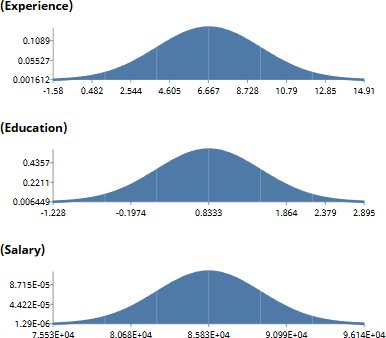
Three variables, three marginal distributions. Experience centered around 6.7 years, Education around 0.8 (slightly below PhD on the modeled scale), Salary around $85K. The shapes describe the population. Nothing has yet been said about how the three relate to one another.
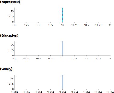
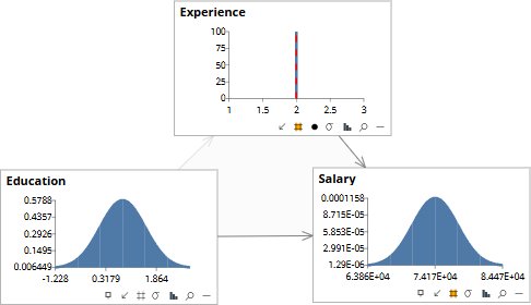
Filter the population to those with Experience ≈ 10. Education collapses to about 0 (no PhD), Salary to about $90K. The conditional distribution is what the data shows: among people with ten years of experience, most have no postgraduate degree and earn well above the population average.
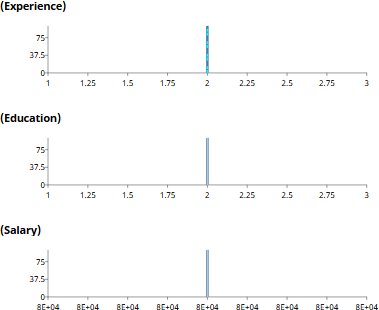
Filter instead to Experience ≈ 2. Now Education collapses to about 2 (well past PhD on the modeled scale), and Salary settles near $80K. The pattern across the two observations is a trade-off: people with little experience tend to have more education, people with more experience tend to have less. Both reach similar salaries by different routes.
Two conditional distributions, two observed patterns. The data has told us what tends to occur with what. It has not told us why. We cannot tell from these panels whether Education causes Experience, Experience causes Education, both are caused by something else (cohort, ability, market timing), or some mixture. We also cannot answer the question a decision-maker actually wants: if we intervened on one of them, what would happen to Salary? No amount of additional observation answers that question. The limit is structural, not a matter of data volume.
This is the ceiling of statistical reasoning and the ceiling of any LLM trained on this data. An LLM can write a long, fluent essay about the relationship between education, experience, and salary. None of that prose breaks the ceiling. The verbosity covers a rung-1 answer in language that sounds like reasoning; it is not. Moving past rung 1 requires adding something the data does not contain: a claim about which variable causes which.
Rung 2 — Doing
The second rung requires structure. Until the causal arrows are drawn, the model cannot distinguish intervention from observation; once they are, it can.
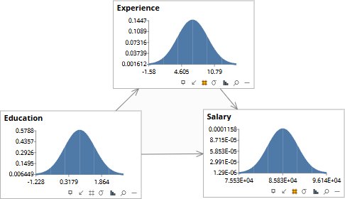
The arrows are cause-and-effect claims. An arrow from Education to Salary asserts that Education is a cause of Salary — that changing Education would change Salary, not merely that the two are correlated in the data. Three arrows are drawn: Education causes Experience, Education causes Salary, Experience causes Salary. The arrows were not inferred from the data — the same correlations would have been consistent with several other arrow assignments. The arrows came from people who know the domain: human capital theory, labor economics, the actual mechanics of how careers produce earnings. This is the value the experts add. The data alone could not have supplied it.
With the structure in place we can intervene: do(Experience = 2). The arrow into Experience is severed for the duration of the intervention — Experience is being imposed, not observed — so Education stays at its prior rather than updating backward. Salary settles around $74,170. Compare this with the rung-1 observation panel: there, observing Experience ≈ 2 gave Salary ≈ $80K. Here, imposing Experience = 2 gives $74K. Different operations, different answers. The intervention bypassed the back-door path Experience ← Education → Salary, giving us the causal answer instead of the observational one.
Rung 3 — Imagining
The third rung asks a question about a specific individual under a counterfactual choice: what would have happened to this person, had something been different? The answer requires more than the structural equations — it requires the idiosyncratic factors that make this person not the average. Pearl gives those factors a name: exogenous noise. Adding the noise nodes turns the Bayesian network into a Structural Causal Model. A Structural Causal Model — SCM — is the diagram plus its equations plus the exogenous noise that makes every variable a complete function of its causes: nothing left unaccounted for.
To make the procedure concrete, take a specific person. This example is Pearl & Mackenzie’s, from The Book of Why (2018, p. 273). Alice has six years of work experience, no PhD, and earns $81,000. Alice’s manager wants to know: what would Alice be earning if she had done a PhD? No population-average answer can address that. The answer depends on who Alice is — the parts of Alice that the structural equations alone do not explain. Those parts are what rung 3 recovers.
Two new nodes appear: Uex (the noise term in the equation for Experience) and Us (the noise term in the equation for Salary). They are sometimes called characteristic variables: they capture what is unique about a specific individual, the parts the structural equations and observable parents leave unexplained. The diagram now records every cause — observed and unobserved — that produces the outcome variables. What we have built is a causal structure, not a statistical summary: the arrows assert which variable causes which, and the equations specify how. This is a Structural Causal Model in Pearl’s sense.
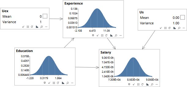
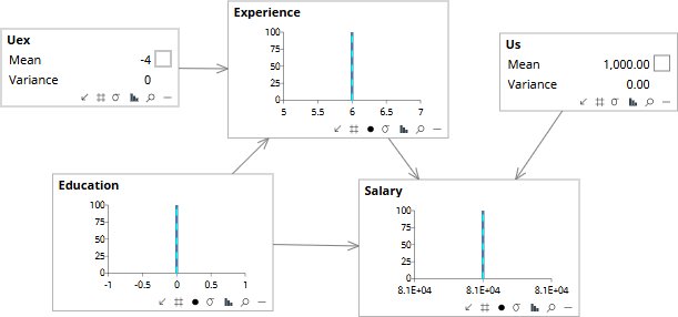
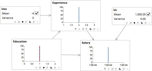
Step one of the three-step procedure. Alice’s observed values — no PhD (Education = 0), six years (Experience = 6), and $81,000 in salary — are entered as evidence. The model runs backward through the structural equations to infer what the characteristic variables must have been to produce these outcomes. Uex = −4 says Alice has four fewer years of experience than the equation would have predicted given her education level; Us = $1,000 says Alice earns about a thousand dollars more than the equation predicts. (The displayed value of Us is in dollars; the prior’s small variance reflects the scale on which Salary deviations live.) These are not population means; they are Alice’s.
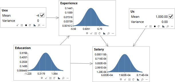
Step two. The characteristic variables are locked at the values from step one (note the checkboxes are now ticked) — this is what makes the result specific to Alice rather than generic — and the original observations on Education, Experience, and Salary are released. The endogenous variables now show the distributions implied by Alice’s abducted noise propagated through the structural equations, with Education back at its population prior. Experience now sits around 0.6 years; Salary around $77K. The model is ready to be asked a counterfactual question with Alice’s idiosyncrasies locked in.
Step three. Education is intervened to PhD (Education = 1) — the counterfactual choice. The model propagates the change forward through the structural equations, with Alice’s abducted noise values still in place, and produces the answer: Experience updates to about 2 years (the PhD would have delayed Alice’s entry into the workforce), and Salary settles near $76,000. Alice would be earning about $5,000 less had she done a PhD. The direct effect of more education is positive, but the indirect effect — the years of work experience Alice would have given up to earn the doctorate — more than offsets it for this specific person. Not the average effect of a PhD across the population; the effect for Alice.
Alice has six years of experience and earns $81,000. Asked what would Alice earn if she had done a PhD?, the three rungs give three different answers:
- Rung 1 — observe. Filter the data to Education = 1 with Experience held at 6: about $85K. This is the wrong answer to use as a counterfactual — it treats the change as an ordinary observation, ignoring that earning a PhD would also have affected how many years Alice could have spent working.
- Rung 2 — intervene on the population. do(Education = 1) across the modeled population gives the average effect of a PhD, with Experience updating to reflect the years of study that took the place of work.
- Rung 3 — counterfactual for Alice. Lock in Alice’s characteristic variables, intervene on Education, propagate forward: $76K. The answer for her.
The manager’s question is a rung-3 question. Rung 1 and rung 2 answer different questions that share the same surface form. The example is from Pearl & Mackenzie, The Book of Why (2018, p. 273).
What changed at each rung
Three structural moves, each unlocking a kind of question the previous rung could not reach:
Added directed arrows. Without them the model cannot distinguish intervention from observation. The arrows are causal claims supplied by domain experts — not inferred from the correlations.
Added exogenous noise nodes. They carry everything the observed parents leave unexplained. Without them the model can answer about populations but not about individuals.
Three steps: abduction (infer the noise from the observed individual), action (lock the noise in and intervene), prediction (run forward to the counterfactual outcome).
None of these moves can be skipped, and none can be made from the data alone. The causal arrows come from experts. The noise nodes come from the modeling formalism. The three-step procedure comes from Pearl. What the data supplies is the conditional distributions that quantify everything else.
An LLM, by itself, is a rung-1 instrument. It is extraordinary at producing fluent text consistent with the statistical patterns in its training data. It cannot, on its own, answer what would happen if we intervened, nor what would have happened for this specific person under a different choice. No amount of additional training data fixes this. The ceiling is structural.
Combine the LLM with a causal model and the ceiling is gone. The natural-language interface stays where it belongs — receiving the question, returning the answer in prose. The causal model handles the part the LLM cannot: it answers rung-2 and rung-3 queries against the structural equations, and returns numbers the LLM can speak. This is what a neurosymbolic system — the architecture Causal AI delivers — looks like in practice. The LLM brings the language; the causal model brings the reasoning. Together they answer questions that neither component could answer alone — and the answers are auditable, because every step is grounded in equations a domain expert can read. The technical accuracy argument →
For the long-form argument about why this matters — why no amount of data closes the gap between rungs without the structure — see What Data Cannot Tell You. For the one-page version, see From the Average to the Case.
A thirty-minute conversation is usually enough to determine whether the questions in front of your decision-makers require a rung beyond the one your current tools were built for.
info@rung3.ai