Why a Causal Model
The Task Force on Climate-Related Financial Disclosures asks organizations to assess and disclose risks across two categories: physical risk (direct financial consequences of climate events — flood, heat stress, wildfire, sea-level rise) and transition risk (financial consequences of the policy, technology, and market changes associated with moving to a low-carbon economy — carbon pricing, stranded assets, shifting consumer demand). TCFD requires scenario analysis: how would a 1.5°C, 2°C, or 4°C pathway affect the organization’s financial position? This is structurally an interventional query — what happens to our financials if we “do” a particular emissions pathway? The risk matrix cannot answer it.
| Analysis Component | Standard Approach | Causal Model | ||
|---|---|---|---|---|
| Scenario analysis | clear | — | ||
| Qualitative narrative — physical and transition risks described, not computed | Forward inference: set Temperature Pathway as evidence, propagate to Net Financial Impact distribution | |||
| Physical risk quantification | clear | — | ||
| Likelihood × impact score for individual hazards, not propagated to financial outcomes | Causal chain from Climate Driver → Hazard → Exposure → Vulnerability → Financial Loss | |||
| Transition risk feedback | clear | — | ||
| Policy and technology treated as independent inputs | Graph encodes co-evolution: carbon pricing accelerates technology adoption; technology reduces political cost of carbon pricing | |||
| Capital allocation | clear | — | ||
| Compliance exercise — no mechanism for linking disclosure to investment decision | VOI analysis identifies which adaptation investments reduce financial uncertainty per dollar |
The ISSB’s IFRS S2 standard (effective 2024) requires quantitative disclosure of climate-related financial risks where material. Qualitative scenario narratives no longer satisfy the disclosure requirement for organizations where climate risk is financially significant. Quantification requires a model. A risk matrix is not a model.
The Questions
- How much of this loss was attributable to a failure to adapt? — Rung 3 (Counterfactual). Answering it requires holding all actual event conditions fixed as observed evidence, changing one prior decision, and computing the difference. The confounder is the specific storm intensity and asset state that must be anchored via abduction before the intervention is applied.
- What will happen to our financials under each TCFD scenario? — Rung 2 (Intervention). do(Temperature Pathway) and do(Policy Scenario) sever the back-door from Geopolitical Context, separating causal scenario effects from the correlations that shared geopolitical drivers create between pathways.
- What is driving our current physical risk exposure? — Rung 1 (Association). Enter Net Financial Impact as observed evidence and read the posterior on Asset Location Risk, Flood Frequency, and Vulnerability to identify which upstream driver is most responsible and which adaptation investment has the highest expected value.
Reading the screenshots: a black check mark on a node means it has been set as observed evidence — a fact entered into the model, acting as a filter. A red check mark means it has been set as a do intervention — a decision applied to the model, severing the influence of its parents.
Reading the spec tables: each Run the Analysis block lists the exact steps to reproduce each screenshot in Bayes Server. The Obs / Do column uses three italic control tokens: clear — reset the model to a blank no-evidence state; abduction step — enter the factual observations that anchor the U nodes to this specific case; use abduction result — apply a do() intervention with the U nodes held from the abduction step.
How much of this loss was attributable to a failure to adapt?
“The flood caused $18M in damage. How much of that would have been prevented if we had built the proposed flood barrier three years ago?”
Rung 2 scenario analysis answers a forward-looking question about a population of future events. This is a narrower question about a specific past event: given everything that actually happened — this storm, this water level, this asset condition — what would the outcome have been if we had made one decision differently? That is Rung 3. It requires abduction first: anchor the model to the actual observed conditions (the specific storm, the actual flood level, the actual asset state) before the counterfactual intervention is applied. Without abduction, you get the average effect of the adaptation across all possible storms — which is a Rung 2 answer to a Rung 3 question, and it will be wrong for this specific event.
The model separates the loss into three counterfactually attributable components: the portion caused by hazard intensity (unavoidable given this storm), the portion caused by asset exposure (reducible by relocation or divestment), and the portion caused by adaptive capacity gaps (reducible by the proposed barrier). In the worked example, anchoring to the actual flood conditions and setting Flood Barrier = Installed reduces expected financial loss by 62% — meaning $11M of the $18M was attributable to the absence of the adaptation, and $7M would have occurred regardless. This framing is what makes a recovery claim against an insurer or a government resilience fund defensible: not “our total loss was $18M” but “our attributable loss from the adaptation gap was $11M, and here is the counterfactual model that produced that figure.”
| Image | Obs / Do | Node | Set | Result |
|---|---|---|---|---|
| esg-prior | clear | — | ||
| — | — | Prior marginals across all nodes | ||
| esg-cf-counterfactual | clear | — | ||
| obs | Flood Frequency | High | ||
| obs | Asset Location Risk | High | ||
| obs | Net Financial Impact | High ($10-20M) | Abduction — PRS and U-nodes anchor to this event | |
| do | Flood Barrier | Installed | Vulnerability shifts: High 27% → 12% |
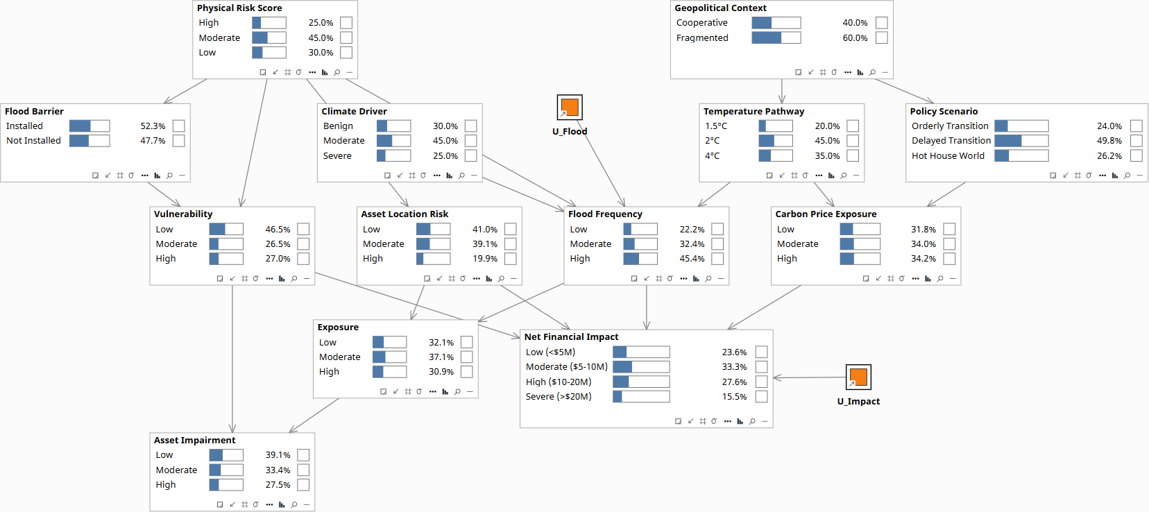
Baseline before any evidence. Prior marginals on Climate Driver, Exposure, Vulnerability, and Net Financial Impact.
Regulatory and litigation exposure increasingly turns on this question. Regulators ask not just whether climate risk was disclosed, but whether the response was adequate given what was knowable at the time — which is precisely a counterfactual over a specific past event. A risk matrix records that a risk was identified. A causal model computes whether the response was prudent, and by how much the outcome would have differed.
What will happen to our financials under each climate scenario?
“Under a 2°C pathway, with current assets and current adaptive capacity, what is our distribution of financial impact?”
TCFD scenario analysis is a forward-looking interventional query: set the temperature pathway and policy trajectory as controlled inputs, then propagate through the causal chain to observe the financial outcome distribution. The risk matrix scores individual risks in isolation — it cannot propagate a scenario through the connected causal structure. The key structural insight for transition risk is that policy trajectory and technology development are not independent: carbon pricing accelerates technology adoption, and technology cost reductions reduce the political cost of carbon pricing. This feedback loop produces qualitatively different scenario distributions than two independent inputs would, and a risk matrix cannot represent it.
The combined physical and transition risk model produces a quantitative distribution of net financial impact for each TCFD scenario — directly satisfying the ISSB S2 quantitative disclosure requirement. Setting Temperature Pathway = 2°C and Policy Scenario = Orderly Transition propagates forward through Flood Frequency and Carbon Price Exposure to Asset Impairment and Net Financial Impact, producing a mean, standard deviation, and tail quantile on Net Financial Impact. The same model run under a 4°C Disorderly scenario produces a materially different distribution — and the gap between them is the financial cost of policy inaction that most qualitative disclosures approximate with a sentence.
| Image | Obs / Do | Node | Set | Result |
|---|---|---|---|---|
| esg-prior | clear | — | ||
| — | Net Financial Impact | Prior distribution across all scenarios | ||
| esg-int-1p5c-orderly | clear | — | ||
| do | Temperature Pathway | 1.5°C | ||
| do | Policy Scenario | Orderly Transition | Low–Moderate loss distribution — ISSB S2 reportable | |
| esg-int-2c-delayed | clear | — | ||
| do | Temperature Pathway | 2°C | ||
| do | Policy Scenario | Delayed Transition | Wider distribution; higher stranded asset exposure | |
| esg-int-4c-hothouse | clear | — | ||
| do | Temperature Pathway | 4°C | ||
| do | Policy Scenario | Hot House World | Fat-tailed physical risk distribution dominates |
Prior distribution across all temperature pathway and policy scenario combinations. Baseline before TCFD scenario is set.
What is driving our physical risk exposure?
“Our expected physical loss is higher than our peers. Which upstream variables are most responsible?”
At Rung 1 the model runs as a filter: enter what you know, read what updates. The graph encodes which dependencies exist — Climate Driver → Hazard → Exposure → Vulnerability → Financial Loss — so setting the financial loss distribution as observed evidence and reading the posterior on root nodes tells you what combination of hazard frequency, asset location risk, and adaptive capacity is most likely driving the outcome. This is the diagnostic direction the risk matrix cannot provide: it can score exposure as “High” but cannot tell you whether the elevation comes from the hazard node, the exposure node, or the vulnerability node — which matters because the remediation is completely different.
Backward inference from an elevated financial loss node identifies the most probable upstream combination — and drives the remediation decision. If the posterior on Asset Location Risk updates strongly while Flood Frequency and Vulnerability stay near prior, the dominant driver is geographic concentration — which points to portfolio rebalancing, not engineering investment. If Vulnerability updates strongly, the driver is adaptive capacity — which points to building upgrades or insurance restructuring. The posterior distribution over root nodes is the capital allocation signal the risk matrix never produces. Running this in reverse also validates the model: if the diagnostically implicated variable is one the organization can measure independently, the model can be updated as new data arrives.
| Image | Obs / Do | Node | Set | Result |
|---|---|---|---|---|
| esg-prior | clear | — | ||
| — | All root nodes | Prior marginals on Climate Driver, Exposure, Vulnerability | ||
| esg-diag-nfi-high | clear | — | ||
| obs | Net Financial Impact | High ($10-20M) | ||
| — | Asset Location Risk | Posterior — compare to prior to identify dominant driver | ||
| — | Flood Frequency | Posterior — hazard-driven vs exposure-driven distinction | ||
| — | Vulnerability | Posterior — adaptive capacity gap if this updates strongly | ||
| esg-diag-alr-high | clear | — | ||
| obs | Asset Location Risk | High | ||
| — | Vulnerability | Near prior — not the driver; remediation = portfolio rebalancing | ||
| esg-diag-vuln-high | clear | — | ||
| obs | Vulnerability | High | ||
| — | Asset Location Risk | Near prior — not the driver; remediation = building upgrades |
Root-cause nodes at prior base rates. No observed evidence entered. Graph encodes which dependencies exist — Climate Driver → Hazard → Exposure → Vulnerability → Financial Loss.
What the Model Enables
Regulatory disclosure
The ISSB S2 requirement for quantitative financial impact disclosure is satisfied by the forward inference: for each IPCC scenario, the model produces a distribution of net financial impact with a mean, standard deviation, and tail risk quantile. This is directly reportable — not a narrative description of risks, but a number with a confidence interval. The same run produces the sensitivity analysis regulators increasingly ask for: which assumption, if changed, most moves the headline figure?
Capital allocation
Running Value of Information analysis across the model identifies which adaptation investments — flood barriers, building upgrades, supply chain diversification, carbon offset purchasing — produce the largest expected reduction in financial risk per dollar of investment. This converts the TCFD disclosure from a compliance exercise into a capital allocation input. The two questions are the same model query run in different directions: forward for disclosure, VOI for capital allocation.
Supply chain resilience
By encoding supply chain nodes as intermediate variables between hazard and financial outcome, the model supports location-specific resilience investment decisions. Which suppliers are in high-risk flood zones? Which logistics nodes concentrate physical risk exposure? The graph propagates these questions to financial consequences — and the do() operator tests the financial impact of each proposed structural change before capital is committed.
Download the Model
The model covers all three rungs in a single file. For Rung 2: set Temperature Pathway and Policy Scenario as do() interventions and read the Net Financial Impact distribution. For Rung 3: observe Flood Frequency, Asset Location Risk, and Net Financial Impact = $18M to abduct the U-nodes, then do(Flood Barrier = Installed). For Rung 1: enter Net Financial Impact = High and read posteriors on Asset Location Risk, Flood Frequency, and Vulnerability.
All models require Bayes Server (free edition available). See Download Models for the full library.
Your TCFD disclosure is a compliance document or a capital allocation tool depending on whether the model behind it can answer “what if?” questions.
The models are free. What I provide is the judgment to build the right structure for your specific situation, encode your experts’ knowledge into it, and turn the output into decisions your board can act on. The discipline stays with your team.