Why a Causal Model
Statistical evidence in criminal trials suffers from a structural problem: the expert answers a question about populations, and the law asks a question about this defendant, this act, this harm. The standard analysis computes P(evidence | guilt) — the probability of observing this evidence if the defendant were guilty. The law requires P(guilt | evidence) — the probability the defendant is guilty given this evidence. These are not the same quantity, and the conversion between them requires a prior probability that the expert must have assumed, implicitly or explicitly. Closing that gap requires moving from Rung 1 — what does the data show? — to Rung 3 — what would have happened if this defendant had acted differently? That is not a statistical question. It is a causal one.
| Analysis Component | Standard Approach | Causal Approach |
|---|---|---|
| Probability direction | P(evidence | guilt) — what the expert computes | P(guilt | evidence) — what the law requires |
| Individual vs. population | Rates across a reference population of cases | This defendant, this incident, this outcome |
| Causation standard | Correlation — presence of DNA, pattern of arrest | But-for counterfactual — would harm have occurred without the act? |
| Confounders | Unmodeled — policing intensity treated as signal | Explicitly separated using the do() operator |
The Questions
- Would this harm have occurred but for the defendant’s act? — Rung 3 (Counterfactual). The but-for test requires holding all actual background conditions fixed and computing the consequence of a changed act. No statistical model can do this without a causal structure; Situational Risk Context is the confounder whose back-door must be closed by abduction before the counterfactual is applied.
- If we intervened to change this defendant’s arrest record, would the risk score change for the right reasons? — Rung 2 (Intervention). do(Prior Arrests) severs the upstream causes of arrest — policing intensity and socioeconomic stress — isolating only the direct effect. The gap between obs() and do() is the confounder the actuarial tool cannot see.
- What does the DNA match actually tell us about guilt? — Rung 1 (Association). The graph encodes P(guilt | evidence), which is what the law requires. The prosecutor’s figure is P(evidence | innocence), which is what the expert computed. Reading the correct posterior from the graph makes the inversion precise and cross-examinable.
Reading the screenshots: a black check mark on a node means it has been set as observed evidence — a fact entered into the model, acting as a filter. A red check mark means it has been set as a do intervention — a decision applied to the model, severing the influence of its parents.
Reading the spec tables: each Run the Analysis block lists the exact steps to reproduce each screenshot in Bayes Server. The Obs / Do column uses three italic control tokens: clear — reset the model to a blank no-evidence state; abduction step — enter the factual observations that anchor the U nodes to this specific case; use abduction result — apply a do() intervention with the U nodes held from the abduction step.
But For Is Rung 3
“Would this harm have occurred but for the defendant’s act?”
Criminal law’s but-for standard is a counterfactual question: hold all background conditions at their actual values, change the defendant’s act, and compute the consequence. Rung 2 gives the average effect of changing an act across all cases like this one. Courts ask a narrower question: given everything that was actually true in this incident, what changes if we change just this one decision? That is Rung 3, and it requires a causal structure to answer.
The model adds a confounder — Situational Risk Context — that independently makes culpable acts more likely and independently elevates harm probability through mechanisms unrelated to the defendant’s choices. This creates a back-door path the observational query cannot close. The three-step counterfactual procedure closes it: abduction anchors the background risk to this incident, then the intervention changes only the defendant’s act while holding that background fixed.
Abduction: obs(Defendant’s Act = At Fault) + obs(Harm = Occurred) + obs(ISC = Absent) — But-For Cause = 92% Yes. The background of this specific incident is now anchored in the U nodes; SRC updates to High 71.8%. Counterfactual: release Harm Outcome, then do(Defendant’s Act = Not At Fault) with U posteriors held. P(Harm = Occurred) drops to 16.1% — the residual hazard from the elevated situational background that exists independently of the defendant’s choices. For comparison, obs(Act = Not At Fault) from the same abducted state gives 13.9%, because obs() allows SRC to infer a lower-risk background — the 2-point gap is the confounding correction. The ISC test from the same abducted state: switching ISC to Present collapses But-For to 70% No, confirming the causal chain breaks when an independent sufficient cause is present.
| Image | Obs / Do | Node | Set |
|---|---|---|---|
| Prior | |||
| but-for-prior | clear | — | But-For Cause: No 68.7% / Yes 31.3% |
| Abduction — anchor the U nodes to this specific incident | |||
| but-for-abduction | clear | — | |
| obs | Defendant's Act | At Fault | |
| obs | Harm Outcome | Occurred | |
| obs | Independent Sufficient Cause | Absent | |
| — | But-For Cause | No 8% / Yes 92% | |
| Counterfactual — change one thing, hold U nodes, read Harm Outcome | |||
| but-for-do | abduction step | — | |
| do | Defendant's Act | Not At Fault | |
| — | Harm Outcome | Occurred 16.1% | |
| but-for-obs | abduction step | — | |
| obs | Defendant's Act | Not At Fault | |
| — | Harm Outcome | Occurred 13.9% | |
| but-for-isc-present | abduction step | — | |
| obs | Independent Sufficient Cause | Present | |
| — | But-For Cause | No 70% / Yes 30% | |
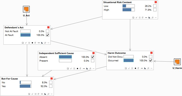
obs(Act = At Fault) + obs(Harm = Occurred) + obs(ISC = Absent). Situational Risk Context updates toward High. U_Act and U_Harm posteriors anchor the background of this specific incident. But-For Cause: 92% Yes.
“Your model is based on historical data from a population of cases. When you say this defendant posed a high risk — was that a statement about this defendant specifically, or about defendants who share certain characteristics with this defendant? These are different things. Did your model compute what would have happened to this defendant if the intervention you’re recommending had been applied to him ten years ago?”
No regression model or actuarial risk tool can answer this. The question isolates exactly what the model cannot do — and what the legal standard requires.
The Confounder in the Witness Box
“If we intervened to change this defendant’s arrest record, would the risk score change for the right reasons?”
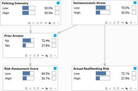
The problem with observational data is that policing intensity and socioeconomic stress both drive prior arrests, so any regression conflates what arrests signal with why they happen. The model separates them using the do() operator: observing an arrest updates its upstream causes because it gives us information about them; setting an arrest by intervention severs that connection entirely, leaving the risk score to rise in the absence of any information about what drove the arrest.
Under do(), Actual Reoffending Risk rises to 40.8%. Under obs(), it stays at 27.9% — unchanged from the prior. The gap is the confounder. When the model observes prior arrests, it cannot update the parents — so Socioeconomic Stress and Policing Intensity stay at their priors and ARR stays flat. When the model intervenes with do(), those parent links are severed and the model updates SES and PI upstream to explain the elevated arrest rate — ARR rises because SES rises. The risk score fires in both cases (High 90%), but in the obs() world it is measuring arrests, not risk. The 13-point gap makes the confounding correction precise and cross-examinable.
| Image | Obs / Do | Node | Set |
|---|---|---|---|
| confounder-prior | clear | — | ARR High 27.9% / RAS High 35.7% |
| confounder-obs | clear | — | |
| obs | Prior Arrests | Yes | |
| — | Risk Assessment Score | High 90% | |
| — | Actual Reoffending Risk | High 27.9% — unchanged | |
| confounder-do | clear | — | |
| do | Prior Arrests | Yes | |
| — | Risk Assessment Score | High 90% | |
| — | Actual Reoffending Risk | High 40.8% — SES updates upstream |
Observing an arrest updates both socioeconomic stress and policing intensity. The graph encodes which dependencies exist — and they flow in both directions.
“Your model uses prior arrest record as a predictor. Did your model account for differences in policing intensity across neighborhoods when computing that score? If two defendants had identical actual behavior but lived in areas with different arrest rates, would your model produce different risk scores for them? Have you tested that? What is the effect size?”
The expert either acknowledges the confounding problem, or claims the model accounts for it — in which case the follow-up is to ask for the mechanism. No standard actuarial tool has this mechanism.
The Prosecutor’s Fallacy
“What does the DNA match actually tell us about guilt?”
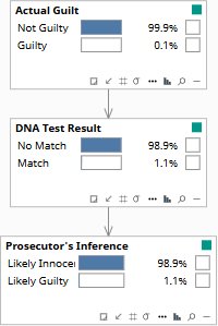
At Rung 1 the model is running as a filter: enter what you know, read what updates. The graph encodes which dependencies exist — Actual Guilt drives the DNA Test Result — so setting DNA Test Result = Match updates the probability of Actual Guilt through that connection. This is where almost all prosecution experts stop, and where the fallacy lives: the expert reports P(match | innocent), and the jury hears P(innocent | match). Bayes’ theorem shows these are radically different quantities.
The correct posterior on Actual Guilt after a DNA match is 9.1% — not 99%. With a prior of 1 in 1,000 (Actual Guilt = 0.1%) and a false positive rate of 1%, a match updates guilt to 9.1% via Bayes’ theorem. The Prosecutor’s Inference node encodes the inverted figure: 100% Likely Guilty. The two nodes sit side by side — 9.1% and 100% — and the cross-examination question writes itself: what prior probability of guilt does your figure assume? The answer is in the Actual Guilt node.
| Image | Obs / Do | Node | Set |
|---|---|---|---|
| prosecutors-fallacy-prior | clear | — | Actual Guilt 0.1% / Prosecutor’s Inference 1.1% Likely Guilty |
| prosecutors-fallacy-match | clear | — | |
| obs | DNA Test Result | Match | |
| — | Actual Guilt | Guilty 9.1% | |
| — | Prosecutor’s Inference | 100% Likely Guilty |
One suspect in a database of 1,000. Before any DNA evidence, the prior probability of guilt is 0.1%.
“Doctor, when you say the probability of a random match is 1 in 10,000 — that is the probability that an innocent person would match the profile, is that right? That is not the same as the probability that this defendant is innocent given the match. Did you calculate the latter? What prior probability of guilt did you use in that calculation?”
Most experts have not done this calculation. The question forces them to either acknowledge the gap or attempt a Bayesian calculation on the stand — which will reveal the base rate they implicitly assumed.
A Cross-Examination Framework
Question 1 — Which probability did you compute?
Force the expert to distinguish between:
- P(evidence | defendant is guilty) — what most experts compute
- P(defendant is guilty | evidence) — what the law needs
These are related by Bayes’ theorem, and the conversion requires a prior probability that the expert must have assumed — implicitly or explicitly. Ask them to state it.
Question 2 — Did your model answer a population question or an individual one?
Statistical models produce answers about distributions. The law asks about individuals. Ask the expert:
- Was your conclusion about defendants with characteristics similar to this defendant, or about this defendant?
- If we intervened to change the factor you identified — not observe it changing, but actually change it — what would happen to this outcome for this person?
- Does your model have a mechanism for that calculation?
Question 3 — What variables did your model not include?
Every statistical model omits variables. Ask the expert to identify the three most important variables their model did not include. Then ask:
- Could any of those omitted variables be correlated with both the predictor and the outcome?
- If so, what is the direction of the bias that omission introduces?
- Has your model been validated in populations with the same distribution of those omitted variables as this defendant?
An expert who has built a structural causal model can answer all three questions. They can show the causal graph, identify which variables are confounders and which are mediators, demonstrate what the counterfactual calculation produces for this specific defendant, and show the sensitivity of their conclusion to the prior probabilities they assumed.
That is not what most forensic statistical experts provide. The gap is not a question of degree — it is a structural gap between two different categories of reasoning.
Download the Model
A single file with three disconnected subgraphs — one per rung. Download, open in Bayes Server, and follow the Run the Analysis steps on this page. The model does the calculation; you observe where the logic breaks.
All models require Bayes Server (free edition available). See Download Models for the full library.
The prosecution’s expert will be cross-examined for thirty minutes. The structural problems in their analysis will have taken years to become embedded in the field. The cross-examination questions are available to any lawyer who understands what the models cannot do.
The models are free. What I provide is the judgment to build the right structure for your specific situation, encode your experts’ knowledge into it, and turn the output into decisions your court can act on. The discipline stays with your team.