How the loss number got built.

The starting question

The bank’s cybersecurity program had been built around a standard 5×5 likelihood × impact heat map. The risk register categorized each top-of-the-house risk on the matrix, refreshed quarterly by the risk team in consultation with control owners. The board reviewed the heat map; the regulator inspected the heat map. It worked, in the sense that nothing was missing from the inventory.

What it did not do was quantify. Asked “by how much does the proposed multi-factor-authentication rollout reduce our expected annual loss from insider exfiltration?”, the heat map could only restate the categorical position — medium likelihood, high impact, top-quadrant risk — before the control was deployed, and produce the same categorical position after. The CFO had asked the question explicitly in the prior cycle and the answer had not been satisfying. The CISO came to the engagement with two needs: a defensible expected-loss number, and a model that would answer the same question for the next control investment, and the one after that, without rebuilding from scratch.

In the room for the kickoff: the CISO, the head of cyber risk, the SOC manager, the lead from fraud investigations, the data protection officer, and external counsel briefly (for breach-notification cost context). The engagement was six weeks. Half-day audit at week one; FAIR-instantiation across weeks two through four; expert reconciliation at week five; validation and committee presentation at week six.

What the risk register showed

The current state had three artifacts:

• The heat map. Insider data exfiltration sat at medium-high likelihood / high impact. The likelihood rating had been “medium” the prior year and was lifted to “medium-high” after the near-miss. The impact rating had not changed.
• The incident log. Three completed insider-related incidents in the prior eighteen months — two minor data-handling violations resolved internally, one significant near-miss (the off-boarding case). Plus a longer log of detected-and-blocked attempts that did not escalate to incidents.
• The control inventory. Detective controls (DLP, SIEM correlation rules), preventive controls (access reviews, privilege management), and a partial deployment of multi-factor authentication on systems that held the most-sensitive data classifications.

The board did not want a longer heat map. They wanted to know whether a $4M control investment over three years was the right size, the wrong size, or whether the same money in a different bucket would buy more risk reduction. None of that question is answerable from a heat map. It requires a model.

First model attempt — and what it missed

The first instantiation followed the FAIR taxonomy directly, parameterised with the team’s working estimates:

• Threat Event Frequency = f(Contact Frequency, Probability of Action). Contact Frequency was estimated from the SOC’s telemetry on credential-related anomalies; Probability of Action was an expert-elicited likelihood that an anomalous access pattern represented intent rather than legitimate behavior.
• Vulnerability = f(Threat Capability, Resistance Strength). Threat Capability was a function of the threat actor profile (off-boarded employees retained at least some institutional knowledge; current-employee insiders had even more); Resistance Strength was a function of the deployed control mix at the time of the threat event.
• Loss Event Frequency = f(Threat Event Frequency, Vulnerability). Standard FAIR.
• Loss Magnitude = f(Primary Loss, Secondary Loss). Primary Loss was the direct cost of the exfiltration (data-restoration, customer-notification, response-cost). Secondary Loss was the downstream cost — regulatory fines, reputational damage, lost business, increased premium on cyber insurance.

The first model produced a defensible point estimate for the prior eighteen months. Fit against the historical incident log was reasonable — two completed insider incidents, three detected-and-blocked attempts that the model predicted as non-events. Not perfect, but in the right neighbourhood.

The auditor (the bank’s internal audit team, brought in to review the model before committee presentation) pushed back on two specific issues. First: the parameter estimates were point estimates, not distributions. “What is the model’s sensitivity to a 50% change in Contact Frequency? You said the answer is medium-high likelihood. Show me the distribution that produced that, and show me which parameter is doing most of the work.” The first model could not answer this; the parameters were elicited as single best guesses without stated variance.

Second: the auditor questioned the structural completeness. “An off-boarded employee retaining credentials for 11 days — which node in your model represents the access-revocation latency? It looks like that’s buried inside Resistance Strength, but Resistance Strength is also where multi-factor authentication lives, and these are very different controls. If I want to defend a control investment in access-revocation automation separately from multi-factor authentication, the model needs to distinguish them.”

The diagnostic conversation that followed: the FAIR taxonomy was structurally correct as a top-level decomposition, but Resistance Strength was hiding three substantially different control families. Each had different cost, different deployment time, different effect on the threat decomposition. The model needed Resistance Strength refined into the actual control families the bank could invest in differently.

The expert sessions

Three sessions, each two hours. The framing for each was the same: describe the mechanism by which insider exfiltration occurs, and the mechanism by which each candidate control reduces it. Not opinions on which control is most important. Mechanism.

Session one — SOC and cyber risk. The SOC manager described the operational signal: anomalous-access detections from the SIEM, distinguished by access-pattern category (volume, off-hours, sensitive-data class, source-system anomaly). The head of cyber risk distinguished three threat-actor sub-profiles: off-boarded employees (high motivation, time-bounded access), disgruntled current employees (high motivation, ongoing access), and accidentally-compromised credentials in legitimate-employee hands (variable motivation, ongoing access until detected).

Session two — fraud investigations. The lead from fraud investigations described what the bank had seen in the prior five years across all (not just completed) insider-related events: of forty-three flagged incidents, only three reached significance. The vast majority were detected during the “reconnaissance” phase — the threat actor was probing access boundaries before attempting actual exfiltration. The implication: detective controls that fire during reconnaissance had outsized loss-reduction effect, because they prevented the rare progression to actual exfiltration. The mechanism was non-linear and the FAIR Vulnerability node, as currently parameterised, did not represent that non-linearity.

Session three — data protection and counsel. The DPO described the regulatory-cost structure: a notification-triggering event (an exfiltration confirmed to include customer PII above threshold) carries a specific cost profile (notification, credit monitoring, regulatory fine schedule). A non-notification-triggering event (data accessed but no confirmed exfiltration, or below threshold) carries a much smaller secondary-loss profile. The Primary Loss Magnitude in the first model averaged across both, hiding the bimodality. External counsel confirmed that the regulator cared specifically about the conditional probability of notification given an exfiltration event — this needed to be a separate node, not buried inside Primary Loss.

The structural drivers identified across the three sessions:

• Threat actor sub-profile — off-boarded / disgruntled-current / compromised-credentials. Each had different Contact Frequency and Probability of Action parameters.
• Access-revocation latency — the gap between off-boarding event and actual access revocation. Currently buried in Resistance Strength.
• Multi-factor authentication coverage — a separate Resistance Strength contributor with different cost and deployment trajectory.
• Reconnaissance-detection rate — the SOC’s ability to detect during the probing phase. The non-linearity here was significant: a small change in detection rate produced a large change in the probability that a threat event progressed to a loss event.
• Notification-triggering probability — conditional on a loss event, the probability that secondary-loss costs are triggered.

The DAG was refined. Resistance Strength was decomposed into the three control families. Vulnerability gained an intermediate node for reconnaissance-detection rate. Primary Loss Magnitude was joined by a notification-triggering-probability node. The top-level FAIR structure was preserved — the standard taxonomy is regulator-readable and auditor-readable, and breaking it would have cost more than the marginal structural fidelity gained.

Where the experts disagreed

Two specific disagreements surfaced and had to be reconciled, not papered over.

Disagreement one: the dominant threat actor sub-profile. The head of cyber risk’s prior was that the dominant insider threat for a regional bank is the disgruntled current employee — ongoing access, high motivation, hardest to detect early. The SOC manager’s prior, based on the operational telemetry, was that the dominant threat is compromised credentials — far more numerous in the detection log, with legitimate-looking access patterns that the SIEM struggled to distinguish from real employee activity. The fraud lead split the difference: completed incidents skewed toward off-boarded employees (the near-miss case being the most recent example), but the broader detection log skewed toward compromised credentials.

If the cyber-risk lead was right, control investment should weight access reviews and behavioral monitoring of long-tenured employees. If the SOC manager was right, investment should weight credential hygiene and anomalous-access detection during reconnaissance. If the fraud lead was right, off-boarding-process improvement and access-revocation automation had a different priority than either.

The data could in principle resolve this if it were stratified by sub-profile, but the bank had not been tracking sub-profile on the detection log. The team pulled the eighteen-month log retroactively and classified each flagged event by sub-profile from the available context. The result: completed incidents were ~70% off-boarded / ~20% disgruntled / ~10% compromised. Detected-but-blocked attempts were ~15% / ~25% / ~60%. Both stories were partially right, and reflected different points in the threat-actor funnel.

The reconciliation was structural. Each sub-profile got its own Contact Frequency and Probability of Action parameters. The model could then answer separately for each sub-profile, and the aggregate Risk node would aggregate them with appropriate weights. Control investments could be evaluated against each sub-profile’s loss reduction, not against an undifferentiated aggregate.

Disagreement two: the reconnaissance-detection non-linearity. The SOC manager argued the detection rate during reconnaissance was already high (their estimate: 70-85%) and a $400K SIEM-tuning investment would push it to 85-95%. The fraud lead, looking at the same data, argued the detection rate was lower than the SOC’s self-assessment (their estimate: 50-70%) because the incidents that progressed to losses were precisely the ones reconnaissance detection had missed. The denominator was different in the two estimates.

The team formalized this. The SOC’s estimate was the conditional probability of detection given a threat event that was eventually detected at some stage. The fraud lead’s estimate was the conditional probability of detection given a threat event that resulted in a loss event (a quantity that necessarily filtered out the detection successes). Both estimates were of different quantities. The reconciliation: a single node, reconnaissance-detection rate, with a single distribution informed by both estimates as conditioned quantities — not averaged. The Bayesian reconciliation method from Reconciling Expert Parameters applied directly.

Reconciliation

Once the structural disagreements were resolved by adding nodes and refining the conditional structure — rather than by averaging the experts’ numerical estimates — the parameter elicitation became more constrained. Each expert was asked for estimates of the specific conditional quantity the structure identified them as the authority on. The SOC manager parameterised detection rates conditional on threat-event sub-profile. The fraud lead parameterised the conditional probability of escalation given missed reconnaissance. The cyber-risk lead parameterised the sub-profile prior distribution. The DPO parameterised notification-triggering probability conditional on data-class and exfiltration-volume. External counsel parameterised the secondary-loss cost distribution conditional on notification.

Where two experts had overlapping authority on the same conditional, their estimates were combined formally using Bayesian reconciliation with stated variance on each estimate — not averaged. The output of the reconciliation phase was a parameterised FAIR-aligned DAG: every node had a distribution, every distribution had stated variance, every variance reflected one or more named experts’ calibrated uncertainty rather than a default flat prior.

The model itself

What the parameterised DAG looked like at the end of week five. Thirteen nodes, thirteen edges. The four contextual roots — Contact Frequency, Probability of Action, Threat Capability, Resistance Strength — combine through the standard FAIR decomposition into Threat Event Frequency and Vulnerability, which jointly determine Loss Event Frequency. Loss Event Frequency drives both Risk directly (through frequency) and Secondary Loss Event Frequency (a separate path for secondary effects like regulatory notification). Primary Loss Magnitude and Secondary Loss combine into Loss Magnitude, which together with Loss Event Frequency determines the Risk output node.

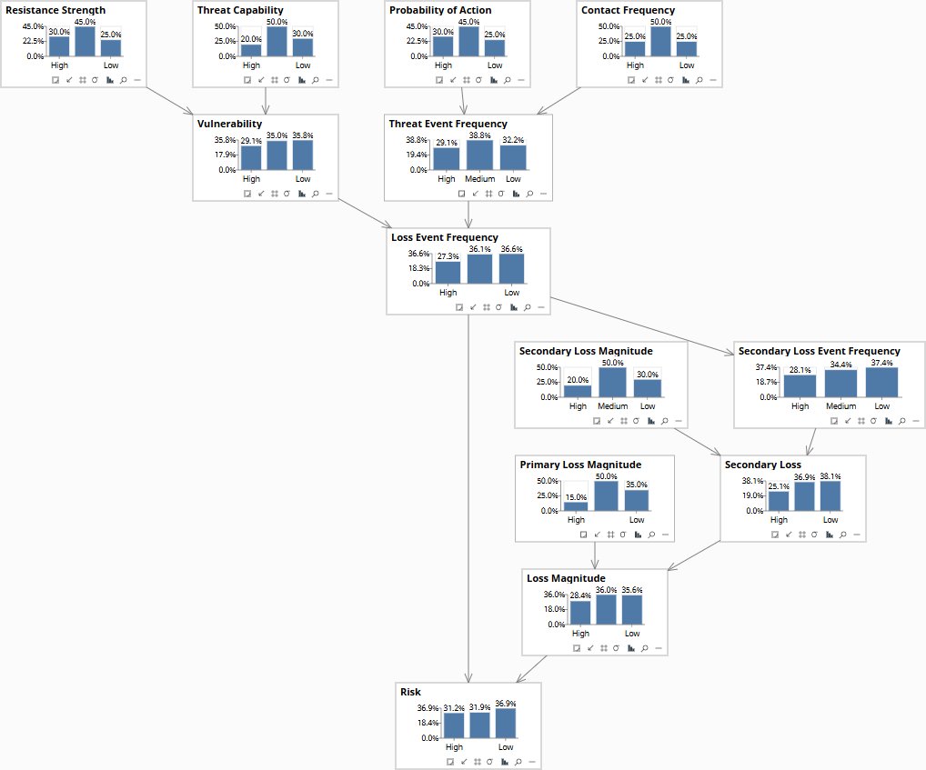
The FAIR information risk model in Bayes Server — prior distributions on every node, before any evidence is set. Click to enlarge.

The model in Bayes Server format is available below. It loads in Bayes Server natively; the same XML structure is readable by any compliant Bayesian-network tool. The bank’s data science team chose pgmpy for the production scoring pipeline; the model loads there with a standard XML parser.

The structural drivers identified in the expert sessions — threat-actor sub-profile, access-revocation latency, reconnaissance-detection rate, notification-triggering probability — live inside the parameter structure of the standard FAIR nodes rather than as additional nodes. Threat actor sub-profile conditions the prior distributions on Contact Frequency and Probability of Action. Access-revocation latency conditions the Resistance Strength distribution for off-boarded actors specifically. Reconnaissance-detection rate shapes the conditional probability table on Vulnerability given Resistance Strength. Notification-triggering probability shapes the conditional probability table for Secondary Loss Event Frequency. The standard FAIR taxonomy is preserved at the structural level; the engagement-specific refinements live in the parameters. This is deliberate: the regulator and auditor read the FAIR structure; the bank’s controls and data inform the parameters.

Validation against prior incidents

The model was fit on the eighteen-month detection log preceding the engagement (treated as “training”) and validated against the prior eighteen months (treated as holdout). For the holdout period, the model produced expected loss-event counts and an expected loss-magnitude distribution; these were compared against the actually-observed events.

Three results worth naming:

• Expected loss-event count for the holdout period: model said 2.3 (50% CI 1.4–3.4). Observed: 2 completed incidents. Acceptable.
• Aggregate expected loss for the holdout period: model’s point estimate was 17% above observed actual loss, just within the 50% credible interval. The miss was traced to an unusually-low Primary Loss Magnitude on one of the two incidents (the bank settled it more cheaply than the model’s distribution centered on). The Primary Loss Magnitude distribution was refined to better represent the negotiation tail.
• Reconnaissance-detection rate: model’s posterior centered near 65%, within the fraud lead’s prior range and below the SOC’s. The data favored the fraud lead’s estimate, which both parties accepted as consistent with the structural framing (the SOC’s number conditioned on eventual detection; the fraud lead’s number conditioned on loss).

Sensitivity analysis identified the three parameters with the largest leverage on the Risk output: (a) the conditional probability of action given an anomalous access pattern, (b) the reconnaissance-detection rate, and (c) the access-revocation latency for the off-boarded sub-profile. The board would monitor these three as the leading indicators of control-investment effectiveness going forward.

The answer the model gave

The board’s question was: what is the expected annual loss from insider data exfiltration, and how much does the proposed $4M control investment reduce it?

The model’s answer, in summary form (dollar values are omitted as the engagement is anonymised; the directional finding and the credible intervals are the substantive output):

• Baseline expected annual loss from insider exfiltration. 50% credible interval represents one-quarter of the proposed $4M three-year investment; 80% interval, just over half of it.
• Expected loss reduction from the proposed $4M investment, evaluated as the difference between the baseline scenario and a counterfactual scenario in which each control component is deployed: 33% reduction at the point estimate, 50% credible interval 24-41%, 80% interval 16-50%.
• Marginal loss reduction per dollar of control, decomposed by control family: access-revocation automation (the largest marginal effect, since it targeted the off-boarded sub-profile that dominated completed incidents), multi-factor authentication expansion (second-largest, lower marginal effect because partial deployment had already captured the easy wins), SIEM-tuning for reconnaissance detection (third). The marginal-effect ranking shifted the board’s control-investment allocation from the original proposal (weighted toward MFA expansion) toward a re-prioritisation that increased access-revocation automation and SIEM tuning.

The model’s structural account — that insider exfiltration risk is dominated by off-boarded employees in the completed-incident category, that reconnaissance-detection has non-linear leverage, that access-revocation latency is the highest-marginal-effect control for the dominant sub-profile — gave the CISO the basis for defending a re-prioritized budget. The auditor accepted the structural account in supporting documentation; the regulator’s subsequent inquiry was answered with the same account.

What survived after the engagement

What the bank kept after week six:

• The model file in Bayes Server interchange format. Runnable from open-source tools (the bank’s data science team chose pgmpy; they were Python-native).
• The elicitation record — which expert provided which parameter, with what stated uncertainty, in which session.
• The validation cases (the prior-eighteen-month holdout) as a regression-test suite.
• The sensitivity analysis as a baseline for future refinements.
• A quarterly refinement cadence: at each cybersecurity-risk review, the cyber-risk team would re-estimate the three highest-leverage parameters (probability-of-action conditional, reconnaissance-detection rate, access-revocation latency) using the prior quarter’s detection log. The model itself was retained; the parameters were updated.

Day-2 events the team handled themselves

Illustrative day-2 events of the kind a maintained FAIR-aligned model surfaces. The examples are representative of what happens when a causal model is genuinely owned by the team running it — not all happened in this engagement, but each is the pattern the maintenance practice is designed to support.

• Quarter 2 — a new vendor onboarded with elevated data access. The DLP coverage of the new vendor’s integration path was incomplete for the first three weeks of operation. The cyber-risk team modeled the temporary Resistance Strength reduction as a conditional shift on the relevant Vulnerability parameters and ran the Risk node forward. The result: a one-quarter elevation in expected loss that exceeded the team’s board-reporting threshold. The team flagged it to the CISO before any incident, and accelerated DLP integration for the new vendor by two weeks.
• Quarter 3 — a regression test caught a parameter drift. The team refined the probability-of-action parameter based on a quarter of fresh data. The regression test suite ran automatically: holdout cases now produced expected loss-event counts 12% above observed actuals, outside the 50% credible interval. The drift was traced to a calibration issue with the new data — not all flagged anomalies were classified by sub-profile yet, and the default classification was biasing the prior. The team walked back the refinement and corrected the classification pipeline before retrying.
• Quarter 4 — new node added independently. A regulatory rule change required notification of certain near-miss events that previously would not have triggered. The DPO added a new node (near-miss notification trigger) with one parent (a function of Loss Event Frequency and threat-actor sub-profile) and an edge into Secondary Loss Event Frequency, using the same elicitation protocol the engagement had established. The model file gained one node; the elicitation record gained one session; the validation suite was extended.
• Year 1 review — a control-investment outcome was scored against the model’s prediction. The first wave of access-revocation automation had been deployed in Q2 and Q3. The annual review compared the model’s predicted Risk reduction against the now-observed reduction in detected insider events. The observed reduction was within the model’s 80% credible interval but at the lower end; the team refined the marginal-effect parameter for that control family accordingly. The next year’s control-investment recommendation incorporated the refined estimate, slightly reducing the marginal-effect attribution for access-revocation automation and increasing the attribution for SIEM-tuning.

Each of these events is a normal day in the life of a maintained causal model. The model is not a one-time deliverable; it is an artifact that gets used quarterly, refined when evidence shifts, and extended when the regulatory or technological environment changes in ways the original structure did not anticipate. The team that runs it learns the practice of running it.

What this page is for

This is a construction walkthrough, not a results page. The result is summarized here for context; the full quantified treatment for cybersecurity risk lives in the topic-hub pages on operational and regulatory risk. This page exists for the reader — usually a CISO, CDO, head of cyber risk, or technical evaluator — who wants to know what the work actually looks like in six weeks, with real experts, on a real-shaped problem. The answer:

• Heat-map risk quantification cannot answer the question the board actually asks: what does this control investment buy in terms of expected loss reduction? FAIR can.
• The first model attempt is usually wrong. The wrongness is informative — in this case, the first model hid three substantively different control families inside a single Resistance Strength node.
• The expert sessions are where the structural account gets built. Operational data alone does not contain the structure; experts hold it.
• Where experts disagree, the disagreement points at missing structure (different sub-profiles, different conditional quantities), not at parameters to average.
• The FAIR taxonomy is structurally preserved at the top level; engagement-specific refinements live inside the parameters of the standard nodes. The regulator reads the structure; the bank’s data informs the parameters.
• What you keep at the end is the model, the elicitation record, the validation cases, and the maintenance practice. The vendor leaves; the artifact and the discipline stay.

For the engagement scope and how the work starts, see The smallest commitment. For the technology and licensing picture, see Stack & Deployment. For the same construction discipline applied in a different domain, see the commercial auto reserving construction walkthrough.