Why a Causal Model
STAR*D, the largest pragmatic trial of antidepressant sequencing, established that approximately one-third of patients remit after a first-line SSRI; among those who do not, approximately a quarter remit at Level 2 (switch or augment); fewer still at Level 3. Those are population averages — the marginal probability of remission at each step, integrated over the heterogeneous population that arrived at that step.
The patient on the table is not the population average. They failed sertraline at Level 1 and venlafaxine at Level 2. Those two specific failures are themselves diagnostic: they tell us something about which kind of depression this is. The history is not a covariate to be controlled for. It is evidence about an unobserved subtype that the next treatment decision needs to condition on.
A standard ML approach to "next-best treatment" would use prior treatments and prior responses as features in a predictive model. That is an associational claim that ignores why those features have the values they do. Treatment_L1 was chosen partly because of demographic and severity covariates AND partly because of the latent type the clinician was already inferring. Response_L1 reflects both Treatment_L1 and the latent type. Conditioning on those features in a regression introduces collider bias on the latent — and the model gives wrong answers for the very decision it was built to support.

Population baseline before any patient evidence.
The Causal Structure
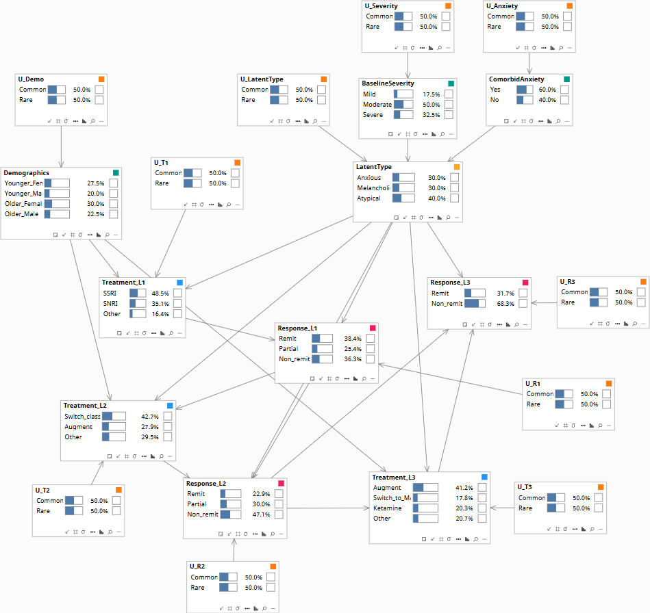
The model is a sequential decision graph with an explicit latent type variable. The latent type is partially observed through baseline severity and comorbid anxiety; it is further constrained by each treatment failure observed in sequence.
| Node | States | Role |
|---|---|---|
| Demographics | Younger_Female · Younger_Male · Older_Female · Older_Male | Pre-treatment covariate |
| BaselineSeverity | Mild · Moderate · Severe | Symptom-derived; informs latent type |
| ComorbidAnxiety | Yes · No | Symptom-derived; informs latent type |
| LatentType | Anxious · Melancholic · Atypical | Latent — never directly observed |
| Treatment_L1 | SSRI · SNRI · Other | First-line agent |
| Response_L1 | Remit · Partial · Non-remit | Updates posterior on LatentType |
| Treatment_L2 | Switch_class · Augment · Other | Second-line agent |
| Response_L2 | Remit · Partial · Non-remit | Further updates posterior |
| Treatment_L3 | Augment · Switch_to_MAOI · Ketamine · Other | The decision under analysis |
| Response_L3 | Remit · Non-remit | Outcome of interest |
Edges encode the structural assumptions: Demographics, BaselineSeverity, ComorbidAnxiety → LatentType (partial observability of the type from observed symptoms). LatentType → all Response_t (response patterns are type-driven). Demographics + LatentType → all Treatment_t (clinicians choose partly based on inferred type). Treatment_t + Response_{t-1} → Response_t (the agent matters; prior failures don't directly cause the next response but their information flows through the latent). Response_{t-1} → Treatment_t (clinicians update).
The latent type makes the treatment-response system identifiable in a way that "control for prior treatments" cannot. The structural form lets the inference engine compute the correct posterior over LatentType after observing the treatment history, then marginalize that posterior when projecting forward. This is what STAR*D's protocol-driven recommendations cannot do — they treat the patient at L3 as a member of the L3 population, not as a specific posterior over types.
The Three Queries
The graph supports three sequential queries — each one a different formal question about the same patient.
How to read the diagrams. An arrow shows the causal direction. An arrow from A to B means A causes an effect — a change — in B.
Two operators appear repeatedly below. obs(X = value) means we learned that X had this value — like filtering the chart-review down to only patients where X was that value. do(X = value) means we imposed this value — like a randomization in a trial, where we control X regardless of what the patient would naturally have. The difference matters: filtering down to "patients who got the drug" tells you something about which patients tend to receive it; imposing the drug tells you only what the drug does.
Among patients with the same demographics, baseline severity, and same prior treatment history who received Augment at L3, what was the remission rate?
Computed as a conditional probability over the data — covariates like Demographics, BaselineSeverity, plus the observed sequence of Treatment_L1, Response_L1, Treatment_L2, Response_L2. Useful for descriptive epidemiology. Polluted by selection: clinicians chose Augment at L3 partly because of suspicions about the patient's LatentType — and that latent state is exactly what we cannot directly observe.
If a fresh clinician with no information about the patient's prior choices were forced to give Augment at L3, what would the remission rate be?
P(Response_L3 = Remit | do(Treatment_L3 = Augment), demographics, severity, anxiety, prior responses). The intervention severs Treatment_L3's dependence on the (unobserved) clinician's inference about LatentType — but the posterior on LatentType, updated by the observed prior responses Response_L1 and Response_L2, still conditions the outcome. This is the right quantity for guideline development.

Population baseline.
This patient remitted at L3 on Augment. Would they have remitted at L1 if mirtazapine had been given instead of sertraline?
The full counterfactual. Abduct the U-values consistent with the factual sequence — Treatment_L1, Response_L1, Treatment_L2, Response_L2, Treatment_L3, Response_L3 — and the inferred LatentType. Intervene on Treatment_L1 to set Mirtazapine; propagate forward; read the counterfactual Response at L1 and beyond. This is the inference that lets the M&M conference — or the malpractice review — assess whether the original treatment plan was reasonable given what was knowable at the time.
Population baseline.
Download the Model
The Bayes Server file below encodes the DAG and the conditional probability tables described above. Each observable node has a corresponding U-node — the exogenous noise variable that absorbs residual variation — which is what makes Rung 3 counterfactual abduction possible. The CPTs are populated with clinically defensible illustrative priors; the qualitative behavior they encode is what makes the failure mode visible when running Rung 1 versus Rung 2 queries on the same data.