Why a Causal Model
A senior adjuster apportions a multi-vehicle claim by constructing a causal chain: which party's action created the conflict point, which determined severity, which eliminated the escape route. She does this for 300 claims. She knows which factors interact, which are legally material in this jurisdiction, and which are noise. A spreadsheet can store her output -- the numbers that came out -- but not the structure that produced them. That distinction is invisible when new claims look like old ones. It becomes visible the first time opposing counsel asks a question the formula was not built to answer.
| Capability | Spreadsheet / Rules Model | Structural Causal Model |
|---|---|---|
| Conditional relationships | Fixed weights applied uniformly | CPTs encode how each factor's weight changes with others |
| Counterfactual answers | Re-runs formula with new input -- not a counterfactual | Abduction fixes background; intervention changes one variable |
| Jurisdiction specificity | One formula or separate sheets with no structural connection | Jurisdiction-specific CPTs on a shared causal graph |
| Audit trail | Formula produces a number; no causal explanation | Every split traceable node by node through the graph |
| Novel fact patterns | Extrapolates linearly from training cases | Probabilistic inference over the causal structure; generalises correctly |
| Deposition readiness | "The adjuster used her judgment" | Point estimate with traceable causal path; auditable at deposition |
| Knowledge retention | Walks out with the adjuster | Encoded in the model; her replacement handles same complexity from day one |
The deposition question is concrete. Try posing it to a frontier language model and see what comes back.
The Questions
- Given everything that was true about this specific collision, would Party B’s fault share have been different if they had been traveling at the speed limit? — Rung 3 (Counterfactual). Answering it requires abduction to anchor the wet road, Party A’s red-light violation, Party C’s tailgating, and the jurisdiction as fixed background conditions before changing only Party B’s speed; Road Conditions and Jurisdictional Standard are confounders that must be held at their actual values.
- What is the causal effect of Party B’s excess speed on fault share, separated from the background conditions that made excess speed more likely in the first place? — Rung 2 (Intervention). A do(Speed = Lawful) query severs the back-door path from Jurisdiction and Road Conditions through driving behavior, isolating the speed decision from the environment that tends to accompany it.
- Given that the collision was severe, what does the model infer about the most probable upstream states — speed, road conditions, visibility, and escape route? — Rung 1 (Association). The graph encodes which dependencies exist between contributing factors and collision severity; entering the observed outcome propagates probability to every connected upstream node in both directions.
Reading the screenshots: a black check mark on a node means it has been set as observed evidence — a fact entered into the model, acting as a filter. A red check mark means it has been set as a do intervention — a decision applied to the model, severing the influence of its parents.
Reading the spec tables: each Run the Analysis block lists the exact steps to reproduce each screenshot in Bayes Server. The Obs / Do column uses three italic control tokens: clear — reset the model to a blank no-evidence state; abduction step — enter the factual observations that anchor the U nodes to this specific case; use abduction result — apply a do() intervention with the U nodes held from the abduction step.
Would Party B's fault share have been different if their speed had been lawful?
“Given everything that was true about this specific collision -- the wet road, Party A's red-light violation, Party C's tailgating, the jurisdiction -- would Party B's fault share have been different if they had been traveling at the speed limit?”
This is the question opposing counsel asks at deposition. It requires individual counterfactual reasoning: not what happens on average when speed is lawful, but what would have happened in this specific collision. The three-step process: abduction (fix this collision's background by updating U nodes from the factual evidence), action (apply do(Party B Speed = Lawful) as an intervention), prediction (compute fault shares with the same U nodes -- the same collision, the same parties, only B's speed changed).
On this specific collision, Party B’s dominant fault band shifts from 75–100% (41.0%) to 0–25% (65.7%) when their speed is made lawful. Collision Severity drops from 93.5% Severe to 58.9% Severe / 41.1% Minor. Liability drops from 71.6% High to 43.4% High. The abduction step anchors the background of this specific collision: U_BS updates to 33.5/66.5 reflecting a driver whose actual choices were consistent with reckless speed in poor visibility. After do(Speed = Lawful), Bayes Server severs all incoming links to the intervention node including U_BS, which returns to its 50/50 prior — this is Bayes Server’s implementation of the do() operator. The remaining evidence (wet road, red light by A, tailgating by C, poor visibility, Modified Comparative jurisdiction) stays in place, and the model computes what fault share would have been for this collision specifically, with only B’s speed changed. Party A’s and Party C’s conduct are unchanged — A still ran the red light, C was still tailgating.
| Image | Obs / Do | Node | Set | Result |
|---|---|---|---|---|
| ia-5-abduction | obs | Visibility | Poor | |
| obs | Road Conditions | Wet | ||
| obs | Party B Speed | Reckless | ||
| obs | Party A Conduct | Red Light | ||
| obs | Party C Conduct | Tailgating | ||
| obs | Jurisdiction | Modified Comparative | ||
| — | U_BS | 33.5% A / 66.5% B — background anchored | ||
| — | Collision Severity | 93.5% Severe / 6.5% Minor | ||
| — | Party B Fault Share | 41.0% (75–100% band) — dominant | ||
| — | Liability | 71.6% High | ||
| ia-6-counterfactual | do | Party B Speed | Lawful | All other evidence held; U_BS severs to 50/50 |
| — | Collision Severity | 58.9% Severe / 41.1% Minor | ||
| — | Party B Fault Share | 65.7% (0–25% band) — dominant band inverts | ||
| — | Liability | 43.4% High — down from 71.6% |
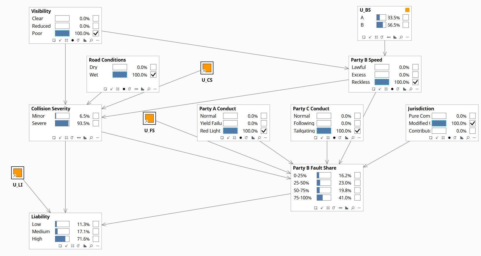
Full fact pattern entered. U_BS updates to 33.5/66.5 — this collision’s driver background is anchored. Collision Severity: 93.5% Severe. Party B Fault Share: 41.0% in the 75–100% band. Liability: 71.6% High.
What is the true causal effect of Party B's speed?
“What is the causal effect of Party B's excess speed on fault share -- separated from the background conditions that made excess speed more likely in the first place?”
Visibility is a confounder for Party B Speed: poor visibility makes excess speed both more likely (drivers misjudge conditions) and more dangerous. When you observe that B was traveling lawfully, Bayes' theorem updates Visibility upward toward Clear -- because lawful speed is more consistent with good conditions. When you intervene on B's speed with do(Speed = Lawful), the link from Visibility to Speed is severed. Visibility stays at its prior. The gap between the two queries is the confounding bias that an observational analysis cannot remove.
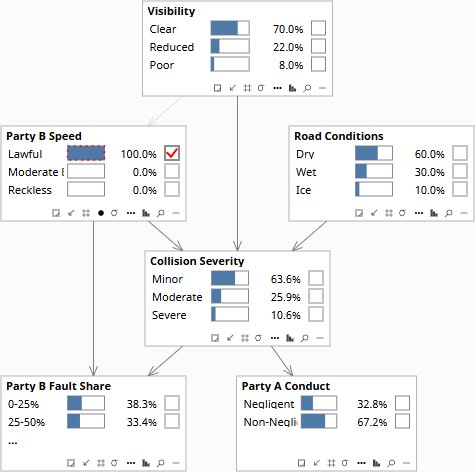
Under do(Party B Speed = Lawful), Visibility stays at prior (70.0% Clear / 22.0% Reduced / 8.0% Poor) and Collision Severity drops to 63.6% Minor / 10.6% Severe. Under obs(Party B Speed = Lawful), Visibility updates to 76.9% Clear / 4.6% Poor — because the model infers that lawful speed is most consistent with good visibility, and the back-door path through Visibility remains open. The Severity and Fault Share numbers are similar in both queries because the confounder gap here is modest (8 percentage points on Visibility). But the direction is exactly as theory predicts — obs() always produces a slightly better Visibility inference than do(), and that inflation compounds through Severity into Fault Share. Any apportionment analysis that conditions on party conduct as evidence rather than intervention carries this bias. The SCM makes the distinction explicit and computable.
| Image | Obs / Do | Node | Set | Result |
|---|---|---|---|---|
| ia-3-speed-do | do | Party B Speed | Lawful | Severs Visibility → Speed link |
| — | Visibility | 70.0% Clear / 22.0% Reduced / 8.0% Poor — stays at prior | ||
| — | Collision Severity | 63.6% Minor / 25.9% Moderate / 10.6% Severe | ||
| — | Party B Fault Share | 38.3% (0–25%) / 33.4% (25–50%) | ||
| ia-4-speed-obs | obs | Party B Speed | Lawful | Back-door open — compare to do() |
| — | Visibility | 76.9% Clear / 18.5% Reduced / 4.6% Poor — updates toward Clear | ||
| — | Collision Severity | 65.2% Minor / 25.2% Moderate / 9.6% Severe | ||
| — | Party B Fault Share | 38.9% (0–25%) / 33.4% (25–50%) |
Visibility stays at prior: 70.0% Clear / 22.0% Reduced / 8.0% Poor. The back-door through Visibility is severed. Collision Severity: 63.6% Minor / 10.6% Severe. Fault Share: 38.3% in 0–25% band. This is the true causal effect of speed, separated from the conditions that made excess speed more likely.
What does this collision's severity tell us about who caused it?
“Given that the collision was severe, what does the model infer about the most probable upstream states -- speed, road conditions, visibility, escape route?”
This is Rung 1 -- diagnostic inference running from observed effect back through the causal graph. The value over a simple correlation analysis is that the graph structure constrains which upstream states are inferred: speed determines severity, not fault; fault is determined by the sequence of actions that created the conflict. A flat correlation model cannot make this distinction. The causal graph can -- and the diagnostic posteriors reflect it.
Setting Collision Severity = Severe updates Party B Speed toward Reckless (44.7% up from 10.0%), Road Conditions toward Wet and Ice (38.7% / 18.7%, up from 32.0% / 10.0%), and Escape Route toward Blocked (55.8% up from 38.0%). Party B Fault Share collapses away from the 0–25% band (4.8%, down from 32.0%) and Liability shifts to 70.9% High (up from 27.8%). The model identifies B’s speed and a blocked escape route as the most likely upstream contributors to a severe outcome — before any party conduct is explicitly known — because that combination is most causally consistent with the observed severity. This is the limit of Rung 1: it tells you where to look. Distinguishing causal effect from confounding requires Rung 2.
| Image | Obs / Do | Node | Set | Result |
|---|---|---|---|---|
| ia-1-prior | — | Party B Speed | 68.0% Lawful / 22.0% Moderate / 10.0% Reckless | |
| — | Road Conditions | 58.0% Dry / 32.0% Wet / 10.0% Ice | ||
| — | Escape Route | 62.0% Available / 38.0% Blocked | ||
| — | Collision Severity | 51.8% Minor / 28.7% Moderate / 19.5% Severe | ||
| — | Party B Fault Share | 32.0% (0–25%) / 29.3% (25–50%) | ||
| — | Liability Assessment | 43.8% Low / 27.8% High | ||
| ia-2-severity | obs | Collision Severity | Severe | |
| — | Party B Speed | 44.7% Lawful / 31.2% Moderate / 24.1% Reckless — excess increases | ||
| — | Road Conditions | 42.6% Dry / 38.7% Wet / 18.7% Ice — adverse conditions update | ||
| — | Escape Route | 55.8% Blocked — up from 38.0% | ||
| — | Party B Fault Share | 4.8% (0–25%) / 14.8% (25–50%) — low bands collapse | ||
| — | Liability Assessment | 70.9% High — up from 27.8% |
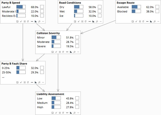
Root nodes at prior: Speed 68/22/10%, Road 58/32/10%, Escape 62/38%. Collision Severity 51.8% Minor / 19.5% Severe. Fault Share 32.0% in 0–25% band. Liability 27.8% High. Enter Severity = Severe to run backward inference.
Download the Models
All models require Bayes Server (free edition available). See Download Models for the full library.
The senior adjuster who knows how to apportion this claim is already counting down to retirement. The conversation identifies the causal structure in her reasoning -- and builds the model that makes it permanent.
The models are free. What I provide is the judgment to build the right structure for your specific situation, encode your experts’ knowledge into it, and turn the output into decisions your board can act on. The discipline stays with your team.