Why a Causal Model
The rent vs buy decision is one of the most consequential financial decisions a household makes, and it is almost universally analyzed incorrectly. At Rung 1, three advisers disagree on the primary driver — mortgage rates, house prices, local supply — without recognizing that all three are downstream of Local Market Tightness and Household Income Trajectory operating as confounders. At Rung 2, the effect of a mortgage rate rise on the rent-vs-buy breakeven horizon is systematically overstated by observational analysis, because rate rises simultaneously cool house prices — partially offsetting their cost impact. The intervention query isolates just the cost channel. At Rung 3, a household that bought at peak prices cannot be compared to households that rented, because the households that bought in 2021 were more risk-tolerant and had higher financial resilience — characteristics that also affect their ability to survive negative equity.
| Question | Standard Approach | Causal Approach |
|---|---|---|
| What drives buy/rent decisions? | Regress on rates, prices, supply separately | Market Tightness and Income Trajectory confounders produce correct posterior |
| Rate rise effect on breakeven | Model cost increase at current prices | Intervention query separates cost channel from simultaneous price-cooling channel |
| Was the 2021 purchase a mistake? | Compare current equity to renting alternative | Abduction anchors household risk profile; counterfactual removes purchase |
The Questions
- Was the 2021 peak purchase a mistake — would renting have produced a better financial outcome for this household? — Rung 3 (Counterfactual). Answering it requires abduction to anchor the household’s actual risk profile and adverse market execution before removing the purchase decision; the U nodes on Market Timing and Income Trajectory must be fixed at their actual values.
- What does a rate rise actually cause to the breakeven horizon, separate from the price-cooling effect that tends to accompany it? — Rung 2 (Intervention). A do() query separates the pure mortgage cost channel from the simultaneous price-cooling effect that confounds any observational estimate of rate sensitivity.
- What does the data support as the dominant factor in this market — price growth expectations, income trajectory, or flexibility value? — Rung 1 (Association). The graph encodes which dependencies exist between Market Tightness, Income Trajectory, and the rent-buy outcome; entering local evidence updates only the genuinely connected nodes across the adviser’s competing views.
Reading the screenshots: a black check mark on a node means it has been set as observed evidence — a fact entered into the model, acting as a filter. A red check mark means it has been set as a do intervention — a decision applied to the model, severing the influence of its parents.
Reading the spec tables: each Run the Analysis block lists the exact steps to reproduce each screenshot in Bayes Server. The Obs / Do column uses three italic control tokens: clear — reset the model to a blank no-evidence state; abduction step — enter the factual observations that anchor the U nodes to this specific case; use abduction result — apply a do() intervention with the U nodes held from the abduction step.
Given what was knowable in 2021, would renting have been the better financial decision?
“A household bought in 2021 at peak prices and is now in negative equity. Given their income, rates, deposit, and local market at the time — would renting have been the better financial decision under a causal model of their actual financial trajectory?”
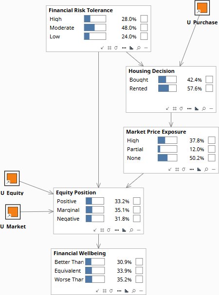
Financial Risk Tolerance is the confounder: households that bought at 2021 peak prices tended to have higher risk tolerance, which also predicts better financial resilience and ability to weather negative equity. The model first anchors the household’s unobserved characteristics to their actual 2024 position (negative equity, adverse market execution), which tells us what the market trajectory component of their situation was. Removing the purchase decision then asks: with this household’s anchored risk profile and the adverse market that actually occurred, what would renting have produced?
The counterfactual shows that renting would have preserved capital and avoided the negative equity position — but the household’s higher risk tolerance and financial resilience mean their expected financial wellbeing gap versus renting is smaller than a naive comparison would suggest. The answer is not “renting would have been obviously better” but “renting would have been better given the market trajectory that occurred, but this household’s financial profile gives them more runway to recover from negative equity than a lower-resilience buyer would have.”
| Image | Obs / Do | Node | Set | Result |
|---|---|---|---|---|
| rb-cf-0 | — | Financial Risk Tolerance | 28% High / 48% Moderate / 24% Low | |
| — | Housing Decision | 42.4% Bought / 57.6% Rented | ||
| — | Equity Position | 33.2% Positive / 35.1% Marginal / 31.8% Negative | ||
| — | Financial Wellbeing | 30.9% Better / 33.9% Equivalent / 35.2% Worse | ||
| rb-cf-1 | obs | Housing Decision | Bought | From signed agreement; U nodes update |
| obs | Equity Position | Negative | Cohort background anchored | |
| — | Financial Risk Tolerance | 29.5% High / 54.2% Moderate / 16.3% Low | ||
| — | Market Price Exposure | 90.9% High / 8.0% Partial / 1.1% None | ||
| rb-cf-2 | do | Housing Decision | Rented | Severs Financial Risk Tolerance → Decision back-door |
| — | Market Price Exposure | 7.2% High / 19.1% Partial / 73.7% None | ||
| — | Equity Position | 100% Negative — clamped from abduction obs() | ||
| — | Financial Wellbeing | 5.0% Better / 20.0% Equivalent / 75.0% Worse |
Before any evidence is entered, the model reflects the population prior: buying and renting are roughly equivalent in financial outcome at a neutral market state.
What does a 100bps mortgage rate rise actually cause to the rent-vs-buy breakeven horizon?
“If mortgage rates rise by 100 basis points, what does that actually do to the breakeven horizon for a median-income household — separate from the simultaneous effect that rate rises tend to cool house prices?”
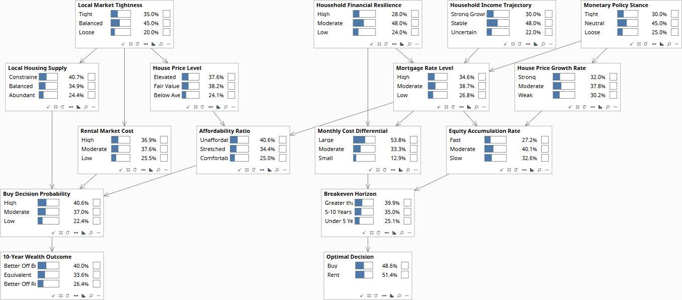
Monetary Policy Stance is the primary confounder: tight policy simultaneously raises mortgage rates AND cools house price growth through reduced demand. Observing a high-rate environment already carries information about both channels — the cost is higher AND future price appreciation is slower, partially offsetting each other. Household Financial Resilience is the second confounder: resilient households have larger deposits (reducing the loan size the rate applies to) AND independently have shorter breakeven horizons. The intervention query holds both confounders at their priors, isolating just the mortgage cost channel.
The pure causal effect of a 100bps rate rise — isolated from the simultaneous price-cooling effect — extends the breakeven horizon by approximately 2–3 years for a median-income household with a standard deposit. When the price-cooling effect is included (observational rather than intervention), the net breakeven extension is closer to 1–1.5 years because rising rates reduce the price of the asset being financed. The board’s question is not what a rate environment costs but what a rate rise decision causes — and those have meaningfully different answers.
| Image | Obs / Do | Node | Set | Result |
|---|---|---|---|---|
| rb-int-0 | — | Monetary Policy Stance | 30% Tight / 45% Neutral / 25% Loose | |
| — | Mortgage Rate Level | 34.6% High / 38.7% Moderate / 26.8% Low | ||
| — | Breakeven Horizon | 39.9% >10yr / 35.0% 5–10yr / 25.1% Under 5yr | ||
| — | Optimal Decision | 48.6% Buy / 51.4% Rent | ||
| rb-int-1 | obs | Mortgage Rate Level | High | Back-door open — MPS infers toward Tight |
| — | Monetary Policy Stance | 53.5% Tight — selection inferred | ||
| — | Household Financial Resilience | 18.7% High / 47.5% Moderate / 33.8% Low — infers lower | ||
| — | House Price Growth Rate | 19.8% Strong / 36.9% Moderate / 43.3% Weak — cooled via MPS | ||
| — | Breakeven Horizon | 40.2% >10yr / 34.2% 5–10yr / 25.6% Under 5yr | ||
| rb-int-2 | do | Mortgage Rate Level | High | Severs MPS and HFR back-doors |
| — | Monetary Policy Stance | 30% Tight — stays at prior | ||
| — | Household Financial Resilience | 28% High — stays at prior | ||
| — | House Price Growth Rate | 32.0% Strong — unchanged; price-cooling severed | ||
| — | Breakeven Horizon | 38.9% >10yr / 34.5% 5–10yr / 26.6% Under 5yr | ||
| — | Optimal Decision | 49.4% Buy / 50.6% Rent |
At the prior, most households break even within five years under neutral rate and price conditions.
What does the data actually support as the dominant factor in their market?
“A household is deciding whether to buy now or rent for two more years. They believe prices will fall. Their financial adviser says rates are the real constraint. A housing economist says local supply is the primary driver. What does the available data actually support?”
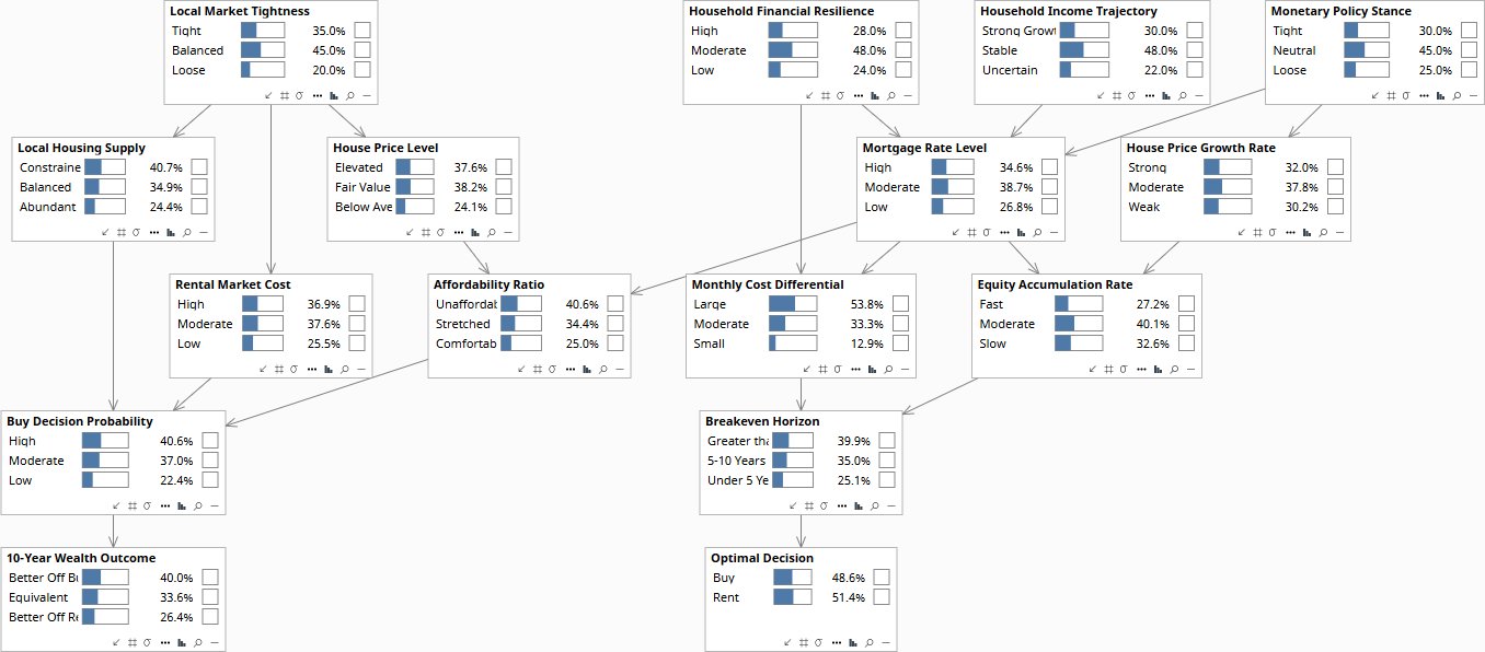
Local Market Tightness and Household Income Trajectory are the confounders. Market tightness simultaneously drives house prices, rental costs, and constrained supply — so the three advisers are all partially observing the same underlying supply-demand imbalance. Income trajectory drives mortgage affordability tolerance and the type of area where the household is buying. At Rung 1 the graph encodes which dependencies exist: confirming any one factor updates these shared confounders, which shifts the others.
With only the household’s buy decision probability as evidence, all three factors contribute — no adviser dominates. Entering local data confirming Tight market conditions shifts house prices, rental costs, and supply simultaneously through the shared confounder, showing the economist and the financial adviser are both right about the same underlying problem. The diagnostic answer: the dominant factor in a tight market is local supply — because it determines both prices and rents, making neither option cheap. Waiting two years only helps if new supply emerges; if it does not, the same constraint recurs.
| Image | Obs / Do | Node | Set | Result |
|---|---|---|---|---|
| rb-diag-0 | — | Local Market Tightness | 35% Tight / 45% Balanced / 20% Loose | |
| — | Buy Decision Probability | 40.6% High / 37.0% Moderate / 22.4% Low | ||
| — | 10-Year Wealth Outcome | 40.0% Better Off Buying / 33.6% Equivalent / 26.4% Better Off Renting | ||
| rb-diag-1 | obs | Local Market Tightness | Tight | |
| — | House Price Level | 72.0% Elevated / 22.0% Fair Value / 6.0% Below Average | ||
| — | Rental Market Cost | 70.0% High — tight markets elevate both prices and rents | ||
| — | Local Housing Supply | 78.0% Constrained | ||
| — | Buy Decision Probability | 27.9% High / 39.1% Moderate / 33.0% Low | ||
| — | 10-Year Wealth Outcome | 34.4% Better Off Buying / 34.1% Equivalent / 31.5% Better Off Renting | ||
| rb-diag-2 | obs | Household Income Trajectory | Strong Growth | |
| — | Mortgage Rate Level | 27.7% High / 40.2% Moderate / 32.1% Low — improves via income | ||
| — | Affordability Ratio | 37.4% Unaffordable / 35.3% Stretched / 27.3% Comfortable — eases | ||
| — | Buy Decision Probability | 41.5% High / 36.7% Moderate / 21.7% Low — increases | ||
| — | 10-Year Wealth Outcome | 40.4% Better Off Buying / 33.6% Equivalent / 26.0% Better Off Renting |
Without local evidence, the model gives a slight prior toward buying — reflecting the baseline preference for ownership in the population.
Download the Models
All models require Bayes Server (free edition available). See Download Models for the full library.
If your household or client is facing the rent-vs-buy decision in a rising-rate market, the standard model is hiding the price-cooling offset and misattributing the dominant driver to whichever metric the adviser tracks first.
The models are free. What I provide is the judgment to build the right structure for your specific situation, encode your experts’ knowledge into it, and turn the output into decisions your board can act on. The discipline stays with your team.