Why a Causal Model
The risk register contained 47 supply chain risks across six categories. Each was scored on likelihood × impact — all marked "managed." There was no row for the scenario where all three suppliers fail on the same Tuesday because all three depended on the same upstream fab. That scenario had a probability near zero if the risks were independent, and near certainty if they weren't. The register had no mechanism to distinguish the two.
| Analysis Component | Standard Scorecard | Causal Model | ||
|---|---|---|---|---|
| Supplier independence | clear | — | ||
| Geographic labels — three countries, three companies | Traces Tier 2 and Tier 3 upstream dependencies; finds shared fab | |||
| Simultaneous failure | clear | — | ||
| Not modeled — risks scored as independent rows | Common-cause nodes encode shared upstream exposure; tail correlation is explicit | |||
| Intervention value | clear | — | ||
| Cannot compute — no mechanism for counterfactual | do(add independent source): 85% reduction. do(add same-fab source): 12% | |||
| Root cause attribution | clear | — | ||
| 5 Whys, fishbone — contributing factors, no causal weights | P(shutdown | no port delay) = 0.72 — port was amplifier, not cause |
The Questions
- What actually caused the $23M loss? — Rung 3 (Counterfactual). Answering it requires holding all actual conditions fixed and computing what would have changed if we had acted differently on each proposed root cause. The post-mortem attribution of the port as a cause required running P(shutdown | do(no port delay)) to test whether removing that factor changed the outcome; Supply Chain Maturity is the confounder that must be anchored before any single-variable counterfactual is applied.
- What will happen if we change our supply structure? — Rung 2 (Intervention). do() separates the causal effect of genuine upstream diversification from same-fab dual-sourcing that shares the dependency and produces only 12% risk reduction at the same cost. The graph distinguishes these two structurally identical-looking decisions; the scorecard cannot.
- Were our suppliers truly independent? — Rung 1 (Association). Entering supply events as observed evidence reveals which upstream nodes update simultaneously, exposing the hidden common causes — TSMC Allocation, Rare Earth Export Policy, Port Congestion — that the scorecard treated as independent rows.
Reading the screenshots: a black check mark on a node means it has been set as observed evidence — a fact entered into the model, acting as a filter. A red check mark means it has been set as a do intervention — a decision applied to the model, severing the influence of its parents.
Reading the spec tables: each Run the Analysis block lists the exact steps to reproduce each screenshot in Bayes Server. The Obs / Do column uses three italic control tokens: clear — reset the model to a blank no-evidence state; abduction step — enter the factual observations that anchor the U nodes to this specific case; use abduction result — apply a do() intervention with the U nodes held from the abduction step.
What actually caused the $23M loss?
“If we had acted differently on each of the proposed root causes, would the stoppage still have happened?”
Rung 2 gives the average effect of changing a supply structure across a population of similar events. The board asked a narrower question: in this specific disruption, with these specific conditions, which factors were genuinely causal and which were amplifiers? That requires holding the actual observed world fixed and asking what would have changed if we had altered just one thing — the definition of a Rung 3 counterfactual.
The port was not the root cause — and the proposed $2M logistics investment would have prevented almost nothing. do(Port Congestion = Normal) left shutdown probability near 49.7%: near the 44.5% prior, confirming the port was an amplifier, not a cause. Qualifying a genuinely independent semiconductor source reduced shutdown probability from 44.5% to 16.4% — a 63% reduction — because it collapsed Semiconductor Availability risk from Allocated 69.6% to 3.8%. Safety stock alone produced only a modest reduction, because a buffer buys time but does not survive a prolonged allocation event. The post-mortem had attributed blame to the wrong variable, and the $2M misdirection was the cost of not running the counterfactual model.
| Image | Obs / Do | Node | Set | Result |
|---|---|---|---|---|
| sc-cf-prior | clear | — | ||
| — | — | Yes 44.5% prior probability | ||
| sc-cf-abduction | clear | — | ||
| obs | Supplier A | Constrained | ||
| obs | Supplier B | Constrained | ||
| obs | Supplier C | Constrained | ||
| obs | Production Stoppage | Yes | U nodes anchored — then release this obs | |
| sc-cf-noport | clear | — | ||
| — | Production Stoppage | released | Query node — read it, do not hold it | |
| do | Port Congestion | Normal | 49.7% — near unchanged | |
| sc-cf-indsource | clear | — | ||
| do | Source Independence | Independent Fab | 16.4% — 63% reduction | |
| sc-cf-buffer | clear | — | ||
| do | Safety Stock | Adequate | 46.7% — modest; not the root cause |
Baseline before any counterfactual is applied. All four proposed root causes at their actual observed states during the disruption.
| Factor | 5 Whys Says | Counterfactual Model Says | ||
|---|---|---|---|---|
| Sole-source semiconductor | clear | — | ||
| Root cause — no alternate existed | do(Source Independence = Independent Fab): P(shutdown) drops from 44.5% to 16.4%. Dominant cause — 63% reduction. Semiconductor Availability Allocated collapses from 69.6% to 3.8%. | |||
| Low safety stock | clear | — | ||
| Contributing cause — only 3 weeks on hand | do(Safety Stock = Adequate): P(shutdown) = 46.7%. Modest reduction alone — buffer buys time but cannot survive a prolonged allocation event. | |||
| Port congestion | clear | — | ||
| External cause — beyond our control | do(Port Congestion = Normal): P(shutdown) = 49.7%. Amplifier, not cause. The semiconductor shortage existed independently of the port. | |||
| Demand spike | clear | — | ||
| Contributing cause — forecast was wrong | Global Tech Cycle (Contraction 74.8% after abduction) is the upstream driver of both demand and TSMC allocation. Structural vulnerability, not forecasting error, was the dominant factor. |
The question of what portion of the $23M loss was caused by the supplier versus own decisions is itself a counterfactual. If a 6-week buffer would have reduced the loss to $7M, the supplier’s causal contribution is approximately $16M — not $23M (total loss) and not $0 (because adequate buffers were not maintained). That framing is what makes a recovery claim defensible.
What will happen if we change our supply structure?
“If we add a second source, or increase buffer stock, or nearshore — what does each intervention actually do to our risk?”
The problem with observational data is that every historical resilience decision was made in a specific supply environment — and that environment does not exist in the new structure. Sourcing from a second supplier sounds like diversification; sourcing from a second supplier that shares the same upstream fab is cosmetic. The causal model tests each proposed change using the do() operator, which severs the incoming arrows to the intervention node and shows only the causal effect of the change, separated from everything that historically accompanied it.
Dual-sourcing from the same fab worsened risk — and genuine independence reduced it by 69%. do(Source Independence = Same Fab) raised Production Stoppage from 44.5% to 55.5%, because forcing all sourcing through a same-fab path concentrates TSMC dependency. do(Source Independence = Independent Fab) dropped it to 14.0%, collapsing Semiconductor Availability Allocated from 30.8% to 2.4%. do(Safety Stock = Adequate) alone produced only a 9% reduction to 40.6% — the buffer absorbs short events but leaves the structural dependency intact. The board’s proposed fix was correct in direction but couldn’t distinguish these outcomes, because it scored the supplier, not the supply chain. The scorecard cannot perform this comparison, because it has no causal graph.
| Image | Obs / Do | Node | Set | Result |
|---|---|---|---|---|
| sc-int-baseline | clear | — | ||
| — | — | Yes 44.5% prior probability | ||
| sc-int-samefab | clear | — | ||
| do | Source Independence | Same Fab | 55.5% — worsens from prior | |
| sc-int-indfab | clear | — | ||
| do | Source Independence | Independent Fab | 14.0% — 69% reduction | |
| sc-int-buffer | clear | — | ||
| do | Safety Stock | Adequate | 40.6% — 9% reduction |

Baseline before any intervention. Sole-source dependency intact. This is the state that produced the $23M disruption.
| Intervention | do(X) | What the Model Computes |
|---|---|---|
| Dual-source critical component | do(Source Independence = Independent Fab) | Production Stoppage drops from 44.5% to 14.0% with truly independent upstream — Semiconductor Availability Allocated collapses to 2.4%. Rises to 55.5% if the second source shares the same fab, because it concentrates more TSMC dependency. The graph distinguishes these — the scorecard cannot. |
| Increase safety stock | do(Safety Stock = Adequate) | Production Stoppage drops only to 40.6% — a 9% reduction. Semiconductor Availability is unchanged; the buffer absorbs short disruptions but cannot survive a prolonged allocation event. Effective as a complement to source independence, not a substitute. |
| Nearshore from Asia to Mexico | do(move supplier from Shenzhen to Monterrey) | Transit risk drops but introduces US—Mexico border exposure. Net reduction depends on whether that profile correlates with the rest of the supply chain. |
| Vertical integration | do(acquire Tier 2 supplier) | Eliminates allocation risk; introduces operational risk. Net effect depends on demand volatility — beneficial in stable demand, costly in volatile. The model computes the crossover point. |
Before investing $5M in dual sourcing, ask: does the decision change if the second source shares upstream dependencies? If it does, that information is worth obtaining first. If buffer stock alone is sufficient regardless, the investigation is unnecessary. This is Value of Information analysis — and it typically saves more than it costs.
Were our three suppliers truly independent?
“When we observe a supply event with one supplier, what updates across the rest of the network?”
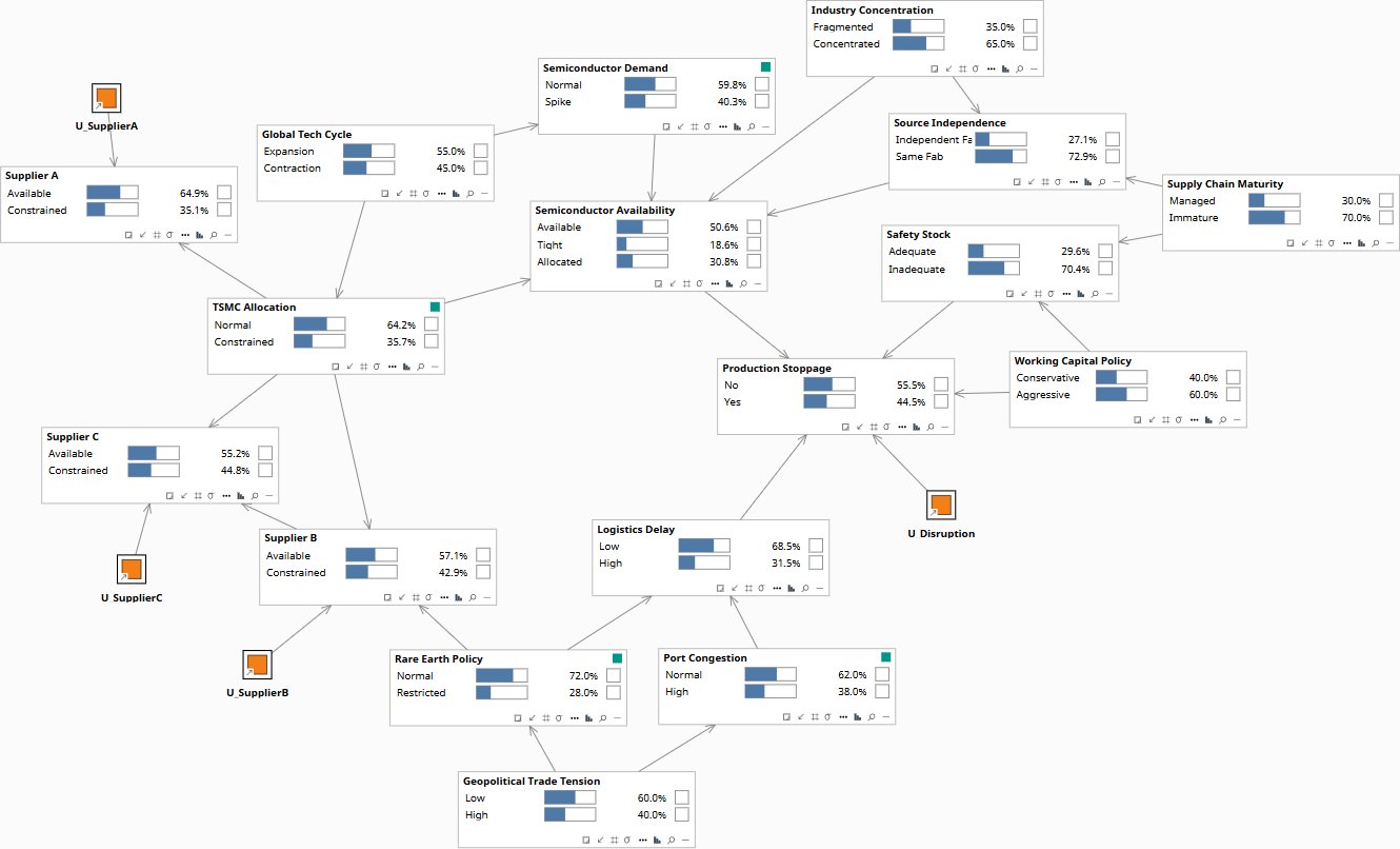
At Rung 1 the model runs as a filter: enter what you know, read what updates. The graph encodes which dependencies exist — and which nodes are genuinely connected through shared upstream causes. When a TSMC allocation event is entered as observed evidence, the model shows which downstream suppliers update and by how much. The scorecard treats each row as independent; the graph reveals which rows are actually one event with three labels.
Observing a TSMC constraint immediately updated all three suppliers simultaneously — because all three traced to the same upstream fab. obs(TSMC = Constrained) pushed Supplier A to 85.5% Constrained, Supplier B to 84.9%, and Supplier C to 92.1% — a full cascade from one piece of observed evidence. Supplier A sourced directly from TSMC. Supplier B sourced through a German broker using the same fab. Supplier C supplied the subassembly that Supplier B required, making it a de facto Tier 2 node on the same dependency chain. obs(Rare Earth Policy = Restricted) revealed a second cascade: Supplier B to 59.7% Constrained, Geopolitical Trade Tension updating to 74.3% High. obs(Port Congestion = High) revealed a third: GTT to 65.3% High, pulling Rare Earth Policy to 38.1% Restricted through the shared confounder. The graph encodes four upstream drivers that create hidden correlation — TSMC Allocation and Global Tech Cycle on the semiconductor side; Rare Earth Policy and Geopolitical Trade Tension on the logistics side — that the scorecard treated as independent rows.
| Image | Obs / Do | Node | Set | Result |
|---|---|---|---|---|
| sc-hc-prior | clear | — | ||
| — | — | Prior marginals — suppliers appear independent | ||
| sc-hc-tsmc | clear | — | ||
| obs | TSMC Allocation | Constrained | Supplier A 85.5%, B 84.9%, C 92.1% — all update | |
| sc-hc-rareearth | clear | — | ||
| obs | Rare Earth Policy | Restricted | Supplier B 59.7%, GTT updates to High 74.3% | |
| sc-hc-port | clear | — | ||
| obs | Port Congestion | High | GTT High 65.3%, Logistics Delay High 61.4% |

Three suppliers appear independent at prior. The graph already encodes the hidden common causes — TSMC Allocation, Rare Earth Export Policy, Port Congestion — the structure is visible before any evidence is entered.
Supply chain risk tools score nodes in isolation. Disruptions propagate through edges. A node-scoring approach is structurally incapable of modeling cascade, correlation, or intervention — because those are properties of connections, not of individual suppliers. This is the same structural problem as The Aggregation Problem — physical rather than financial, but the mathematical failure is identical.
Twelve Months Later
The team qualified a single genuinely independent semiconductor source — a Korean fab with no TSMC upstream exposure and a different logistics corridor. They increased buffer stock to six weeks on the critical component. Total investment: $3.1M across qualification costs, buffer stock, and working capital.
In the twelve months following, four disruption events that would previously have reached the production line were absorbed:
| Event | Previous Outcome (estimated) | Actual Outcome | Saving | |
|---|---|---|---|---|
| TSMC allocation reduction, Q1 | clear | — | ||
| 12-day stoppage | Korean source covered 100% of shortfall | $4.1M | ||
| Rotterdam port slowdown, Q2 | clear | — | ||
| 5-day delay | 6-week buffer absorbed entirely | $1.9M | ||
| Supplier B quality hold, Q3 | clear | — | ||
| 8-day partial stoppage | Korean source + buffer: no line impact | $1.7M | ||
| Malaysian logistics disruption, Q4 | clear | — | ||
| 3-day delay | Rerouted through German corridor | $0.7M |
The Bottom Line
- The scorecard said "three independent suppliers." The model said "one fab, three labels." The model was right.
- The proposed fix (dual-sourcing) was correct in direction but would have delivered 12% risk reduction. The right fix delivered 85%.
- The port was not the root cause. Counterfactual analysis prevented $2M in misdirected logistics investment.
- $3.1M investment. $8.4M recovered in year one. Payback in 4.3 months.
Download the Models
Each model is the formal structure underlying one of the three questions on this page. Download, set evidence on any node, run inference. The model does the calculation — you observe where the scorecard was wrong.
All models require Bayes Server (free edition available). See Download Models for the full library.
Every manufacturer has a critical path where the scorecard says “managed” but the team knows a single failure cascades. The causal model finds that path — and quantifies what it would cost to move it.
The models are free. What I provide is the judgment to build the right structure for your specific situation, encode your experts’ knowledge into it, and turn the output into decisions your board can act on. The discipline stays with your team.