The bridge tool, file by file: four components, ~2,500 lines of R and Python.

Architecture

The bridge is a four-stage pipeline. Each stage takes a structured object from the previous stage, transforms it, and hands it to the next. Components are deliberately decoupled: each can be tested, replaced, or extended independently.

What the bridge adds beyond Robyn

Robyn produces a regression fit. The bridge adds three things the regression doesn't have:

1. An explicit LatentDemandState confounder. A root node with arrows to all media channels and to Sales. The back-door Robyn assumes away. Strength is parameterized as λ so the analyst can sweep it.
2. U-noise parents on every substantive node. Required for Rung-3 (counterfactual) inversion via twin networks. Each U_X node is a unit-variance Gaussian root that captures the unexplained variance of its substantive partner.
3. Linearized media coefficients. Robyn's Hill saturation is non-linear; linear-Gaussian SCMs are linear by construction. The bridge linearizes around the operating point (mean weekly spend per channel). The marginal coefficient at current spend is preserved exactly.

Why closed-form math, not Bayes Server runtime

The constructed SCM is fully linear-Gaussian. All three Pearl-ladder queries — observation, intervention, counterfactual — reduce to standard linear algebra and have exact closed-form posteriors. Component 3's R implementation matches what Bayes Server's exact inference engine would compute on the same .bayes file. The runtime isn't needed; the file is the auditable artifact.

For non-Gaussian extensions — Poisson sales, mixed discrete/continuous nodes, hierarchical pooling, full DBN unrolling for adstock — Bayes Server's runtime via rJava becomes the right backend. The current implementation doesn't need it. A future production version would.

Component 1 — Reader

Public API

# Read a Robyn fit JSON and extract bridge inputs
read_robyn_fit(json_path) → BridgeInputs

# Print a human-readable summary
print(bridge_inputs)

# Audit for missing fields before passing to Component 2
audit_bridge_inputs(bridge_inputs) → character vector of issues

# Convert to a plain list (drops S3 class) for serialization
bridge_inputs_to_list(bridge_inputs) → list

Defensive parsing — sample

The most fragile part of Component 1 is the per-channel summary extraction. Robyn 3.12.1 stores per-channel data in ExportedModel$summary as a data frame, but the column names changed at some point — older versions used rn for variable name, newer use variable. The reader handles both:

channel_summary <- function(ch) {
  # Find the row by variable name. Robyn 3.12.1 uses 'variable';
  # older versions used 'rn'. Try both.
  name_col <- if ("variable" %in% names(summary_df)) "variable"
              else if ("rn" %in% names(summary_df))  "rn"
              else NULL
  if (is.null(name_col)) return(empty)

  row <- summary_df[summary_df[[name_col]] == ch, , drop = FALSE]
  if (nrow(row) == 0) return(empty)

  list(
    coef           = pick("coef"),
    total_response = pick("decompAgg") %||% pick("xDecompAgg"),
    roi            = pick("performance") %||% pick("roi_total")
                                          %||% pick("roi_mean"),
    boot_mean      = pick("boot_mean"),
    ci_low         = pick("ci_low"),
    ci_up          = pick("ci_up")
  )
}

The %||% coalescing operator and the pick() helper that returns NA for missing fields keep the reader resilient: a JSON missing one field doesn't crash the whole pipeline, it just produces a BridgeInputs with that field as NA. The audit function then surfaces missing fields explicitly so Component 2 doesn't silently consume incomplete input.

Full file: R/bridge_reader.R · Documentation: docs/bridge_reader_README.md

Component 2 — SCM Constructor

The structural correction formula

The associational-to-structural translation is parameterized as a linearized Gaussian back-door correction. For each paid channel:

At λ=0 the bridge agrees with Robyn (no confounder asserted). At λ=1 the bridge applies full back-door correction. Calibrated channels (those with experimental anchors) get attenuated lambda by 70% — the experiment partly blocks the back-door, so the correction shouldn't double-count.

Per-channel back-door strengths

Component 2 accepts latent_to_media as either a scalar or a named list. The named-list form lets the analyst specify different back-door strengths per channel — TV with 0.7 (advertisers heavily plan TV around demand forecasts) and Search with 0.0 (search is more demand-driven on the user side, less planning-driven on the advertiser side):

build_scm_from_robyn(
  bridge_inputs   = br,
  output_path     = "./robyn_outputs/bridge_scm.bayes",
  lambda          = 1.0,
  latent_to_media = list(
    tv_S     = 0.7,    # upfronts-locked planning, strong back-door
    search_S = 0.0     # demand-bid auctions, weak back-door
  ),
  latent_to_sales = 0.5
)

This is the kind of judgment call a configurator playbook elicits during week 2 of a real engagement. The current implementation defaults to a uniform 0.7 across all paid channels for the demo dataset.

What gets emitted

The output .bayes file is a self-contained Bayes Server network. For the synthetic demo dataset (2 paid channels, 1 organic, 3 controls), it has 12 nodes and 13 links: the LatentDemandState root, U-noise nodes for each substantive variable, the Sales outcome with structural coefficients, and the context variables as observable inputs. The file is openable in Bayes Server desktop for independent inspection.

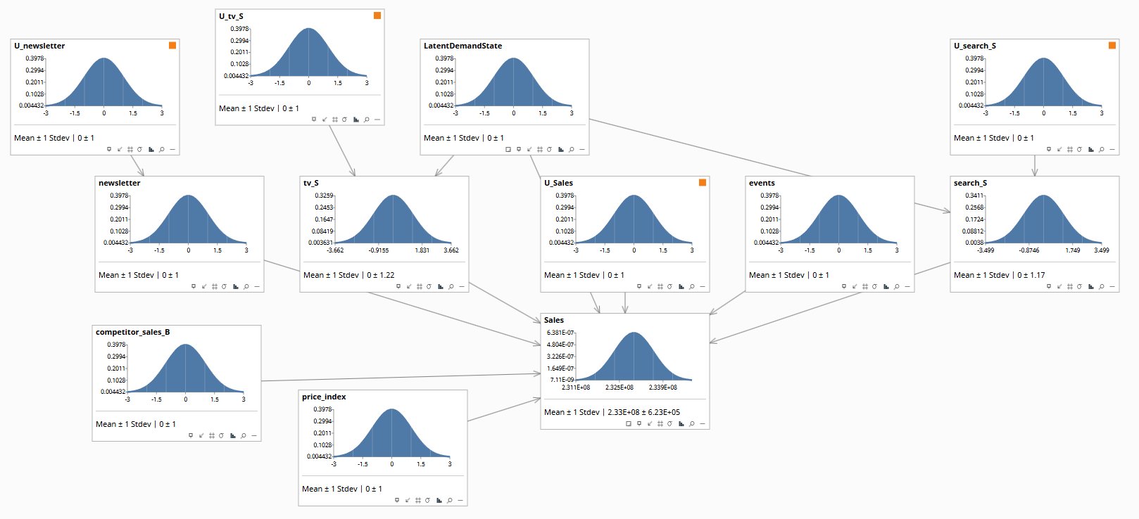
The bridge-constructed SCM in Bayes Server desktop. Each node is shown with its marginalized distribution. LatentDemandState sits at top — the back-door confounder Robyn doesn't model. Orange flags mark the U-noise parents required for Rung-3 counterfactual inversion. Media channels (tv_S, search_S, newsletter) receive arrows from both the latent and their U-noise. Sales at bottom-right shows the marginalized outcome (~$233M ± $623K at zero evidence), with structural coefficients on every incoming arrow. The latent-strength parameters driving the bridge's correction — latent_to_media per channel, latent_to_sales, lambda — are domain-elicited rather than measured. Elicitation is hard; the bridge doesn't eliminate the problem, it parameterizes it so the assumptions can be made explicit and sensitivity-tested via the Shiny app's sliders.

Full file: R/bridge_constructor.R · Documentation: docs/bridge_constructor_README.md

Component 3 — Query Runner

The three queries

Pearl's ladder distinguishes three classes of question, each requiring more structure than the last:

• Rung 1 — Observation. E[Sales | observed(spend = X)]. The data-conditional expected Sales. What Robyn already reports. Component 3 reproduces it as a sanity check.
• Rung 2 — Intervention. E[Sales | do(spend = X)]. The structural effect of intervening on spend, with all back-door paths cut. The bridge's headline output.
• Rung 3 — Counterfactual. E[Sales* | observed evidence, do(spend* = 0)]. Per-campaign attribution. Given a specific observed period, what fraction of the lift is causally attributable to the campaign vs. would have happened anyway?

Closed-form computation — sample

The Rung-2 (intervention) query is the cleanest: do() cuts inbound arrows to the intervened node, so the latent demand state and other roots return to their unconditional means (zero), and only the direct structural effect contributes:

query_rung2 <- function(scm_rf, channel, do_value, structural_coef) {
  # In a do-intervention, all upstream paths to <channel> are cut.
  # The latent demand state and other roots return to their
  # unconditional means (zero), and only the direct structural
  # effect of <channel> on Sales contributes — at level
  # structural_coef * do_value.
  expected_sales <- scm_rf$base_sales + structural_coef * do_value

  list(
    channel                  = channel,
    do_at                    = do_value,
    expected_sales           = expected_sales,
    expected_lift_per_dollar = structural_coef
  )
}

Rung 3 is more involved — it requires the abduction step (posterior on root variables given the observed evidence) followed by the action step (apply the intervention in a twin network) and the prediction step (compute the outcome). All three steps are closed-form for linear-Gaussian SCMs; the implementation is about 30 lines.

Lambda sweep — the sensitivity-chart data

sweep_lambda(
  bridge_inputs   = br,
  output_dir      = "./robyn_outputs/sweep",
  lambdas         = seq(0, 1.4, by = 0.05),
  latent_to_media = 0.7,
  latent_to_sales = 0.5
) → # tidy dataframe: lambda, channel, robyn_roi, structural_roi

This rebuilds the SCM and reruns Component 3 at 29 lambda values from 0 to 1.4. On a recent laptop the full sweep takes 1–2 seconds. The Shiny app calls this on every parameter change to refresh the sensitivity chart.

Full file: R/bridge_queries.R · Documentation: docs/bridge_queries_README.md

Component 4 — Shiny App

The reactive graph

# On startup (cached for app lifetime)
BRIDGE_INPUTS <- read_robyn_fit(ROBYN_JSON)

# On every parameter change (slider drag)
l2m_list <- reactive({
  # Per-channel latent_to_media as a named list, from the dynamically
  # rendered per-channel sliders
})

scm_current <- reactive({
  build_scm_from_robyn(BRIDGE_INPUTS, tempfile(),
                       lambda = input$lambda,
                       latent_to_media = l2m_list(),
                       latent_to_sales = input$l2s)
})

queries_current <- reactive(run_bridge_queries(scm_current()))

sweep_current <- reactive({
  sweep_lambda(BRIDGE_INPUTS, tempdir(),
               lambdas = seq(0, 1.4, by = 0.05),
               latent_to_media = l2m_list(),
               latent_to_sales = input$l2s)
})

Each plot's renderPlot() depends on either queries_current() or sweep_current(), so dragging a slider invalidates the relevant reactive and triggers a chart redraw. The cascade is automatic — Shiny handles the dependency graph.

What the analyst actually sees

Four tabs, each addressing one job:

• Headline. Side-by-side bar chart of Robyn ROI vs bridge structural ROI per channel, with truth lines (where known) for sanity. The single most important screen.
• Sensitivity. The lambda sweep — solid curves of bridge correction as λ goes from 0 to 1.4, dotted lines for Robyn's reported ROIs, vertical line marking current λ slider position.
• Counterfactual. Stacked bars decomposing observed weekly sales into "would have happened anyway" vs "campaign-attributable" for a high-spend week.
• Export. Download buttons for the current .bayes file, the audit CSV, and the lambda-sweep CSV.

Full file: R/app.R · Documentation: docs/app_README.md

Running it end-to-end

The full pipeline reproduces in roughly fifteen minutes on a multi-core laptop, ten of which are Robyn's hyperparameter search. Everything else is fast.

Prerequisites

• R 4.3+ with Rtools (Windows) or build-essential (Linux/Mac)
• Python 3.11+ for synthetic-data generation
• Robyn package: install.packages("Robyn") — see Robyn's docs for full setup including the Python venv with nevergrad

Reproducing the worked example

# Generate synthetic dataset (Python)
python python/build_mmm.py
python python/build_robyn_dataset.py

# Fit Robyn (R, ~10 min on a multi-core laptop)
Rscript R/robyn_run.R

# Run the bridge end-to-end (R, instant)
Rscript -e '
  source("R/bridge_reader.R")
  source("R/bridge_constructor.R")
  source("R/bridge_queries.R")
  br <- read_robyn_fit("./robyn_outputs/RobynModel-3_121_9.json")
  scm <- build_scm_from_robyn(br, "./robyn_outputs/bridge_scm.bayes",
                              lambda = 1.0)
  print(run_bridge_queries(scm))
'

# Or launch the Shiny app
Rscript -e 'shiny::runApp("R/app.R")'

Expected output

On the synthetic dataset, where the structural truth is knowable in advance, Robyn reports inflated TV ROI ($2.83 vs truth $2.00, +41%); the bridge recovers TV within 8% of truth at λ=1.0 with latent_to_media=0.7. Search shows the methodology's limit honestly: Robyn's regularization shrinks Search below truth, and the bridge can correct back-door bias but not regression shrinkage upstream. See outputs/mmm_three_rungs_analytic.txt in the repository for the closed-form analytic reference.

The repository

All four components plus the synthetic data, the standalone SCM, the Robyn fit script, and per-component documentation live in a single repository. MIT-licensed, open for clone, fork, or extension.

Repository structure

What's not in the repo (yet)

Three things a production version would need that the current implementation doesn't have:

• Joint refitting. The bridge currently corrects Robyn's already-fit coefficients. A more rigorous version would refit the model with the SCM structure baked in from the start, avoiding the regularization-shrinkage limit shown by the Search channel.
• Hierarchical pooling. Multi-geo, multi-brand, partial pooling — the bridge handles single-geo only. Hierarchical extensions are tractable but require more SCM structure.
• Non-Gaussian likelihoods. Poisson sales, truncated-normal spend, mixed discrete/continuous nodes. These break the closed-form math and require Bayes Server's runtime via rJava — the right backend for production use.

Each of these is a real engineering project, not just a config knob. The current implementation demonstrates the methodology works on a synthetic linear-Gaussian dataset; production extensions are where the consulting engagement adds value beyond the open-source code.