The structural causal model for resilience justification: explicit confounders, three rungs, closed-form posteriors.

The SCM for buffer-inventory resilience

The question — "did our pre-disruption buffer-inventory investment pay off during the disruption?" — has a specific structural shape. Three classes of variable need to be in the model:

• The decision under question. Buffer investment, in standardized weeks-of-cover. The treatment we want to attribute outcomes to.
• The latent confounders. Two of them. MarketState drives both demand environment and the firm's resilience stance; ResiliencePosture is the firm-level latent that drives buffer decisions and (separately) drives stockout outcomes through other channels.
• The outcomes. StockoutLoss (revenue lost during the disruption), CarryingCost (the cost of holding the buffer), and NetBenefit = −StockoutLoss − CarryingCost as the headline.

Plus a co-decision (MultiSourcing) that's typically made alongside buffer and gets confounded with it; including it lets us isolate buffer's specific causal effect from the broader resilience program.

The structural equations

All variables standardized to mean 0, scale 1. Disruption severity is fixed at 1.5 (calibrated against publicly-observed Q1 2020 magnitudes for consumer-goods supply-chain disruptions). The buffer-effect coefficient on stockouts is therefore 0.8 × 1.5 = 1.20 at this severity:

MarketState (M)        ~  N(0, 1)
ResiliencePosture (R)  =  0.6·M + U_R              [confounded by market state]

BufferInvestment (B)   =  0.5·M + 0.7·R + U_B      [the back-door: market and
                                                    posture both drive buffer]
MultiSourcing (MS)     =  0.4·M + 0.6·R + U_MS

StockoutLoss (SL)      =  3.0                      [base disruption loss]
                          − 1.20·B                 [buffer reduces stockouts]
                          − 0.75·MS                [multi-sourcing reduces too]
                          − 0.30·R                 [posture reduces independently]
                          + U_SL

CarryingCost (CC)      =  0.40·B + U_CC

NetBenefit (NB)        =  −SL − CC                 [headline]

True direct effects (what Rung 2 will recover):

• Buffer's effect on StockoutLoss reduction = −1.20 per standardized unit
• Buffer's effect on CarryingCost increase = +0.40 per standardized unit
• Buffer's net effect on NetBenefit = +0.80 per standardized unit

Why this DAG and not another

The DAG embeds three claims that should be inspected before any analysis:

1. MarketState confounds everything. Firms in a more volatile market environment invest more in resilience AND face larger disruptions. Without conditioning on this, observed correlations between buffer and outcomes absorb the market effect.
2. ResiliencePosture is the second confounder. Firms with stronger posture invested more in buffer AND had better outcomes for non-buffer reasons. This is the cleaner of the two confounders — it's domain-elicited rather than purely statistical.
3. The buffer's effect is conditional on disruption. In the model, the buffer reduces stockouts only when the disruption hits. We've encoded this by fixing disruption severity at 1.5 throughout the dataset, which collapses the interaction term B × D to a linear coefficient at that severity. Sensitivity to disruption severity is exposed via the Shiny app rather than re-fitted in the SCM.

Each of these is a configurator decision in a real engagement. The data-generating process here represents a defensible default; a configured-for-client version would adjust the latent strengths based on industry, geography, and the client's actual planning process.

U-noise nodes

Each substantive variable has a unit-variance Gaussian noise parent (U_R, U_B, U_MS, U_SL, U_CC). These are required for Rung-3 (counterfactual) inversion via the twin-network procedure: we need to be able to abduct the noise terms from observed evidence, then re-run the model under intervention with those noise terms held fixed. Same convention as the MMM standalone SCM.

The SCM as Bayes Server renders it

The structural equations above, encoded as a CLG (Conditional Linear Gaussian) network in ResilienceInvestment-AllRungs.bayes and opened in Bayes Server desktop:

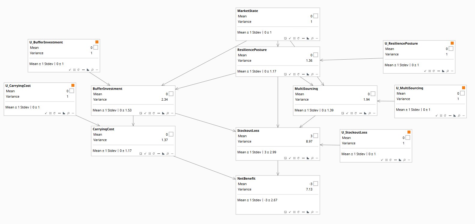
The constructed SCM in Bayes Server desktop. Each node shows its marginal distribution at zero evidence. MarketState at top is the latent confounder; orange-flagged U-noise nodes are unit-variance Gaussian roots required for Rung-3 inversion. The marginal StockoutLoss of 3.0 ± 2.99 is the disruption base loss before mitigation, and NetBenefit at the bottom shows the headline marginal of −3.0 ± 2.67 — the firm loses approximately 3.0 standardized units to a Q1 2020-magnitude disruption when neither buffer nor multi-sourcing is invested. The Pearl-ladder queries in the next section adjust this baseline as buffer and posture conditions change. The latent-strength parameters that drive these adjustments — how much the firm's resilience posture shaped its buffer decision, how much market state independently affected outcomes — are domain-elicited rather than measured. Elicitation is hard; the SCM doesn't eliminate the problem, it parameterizes it so the assumptions can be made explicit and sensitivity-tested.

Pearl's three rungs on this question

For the resilience question, each rung answers a structurally different version of "what did the buffer buy us":

The Rung-1-vs-Rung-2 gap (−1.68 − (−3.00) = +1.32 for naive vs −2.20 − (−3.00) = +0.80 for structural) is the headline naive-analysis bias: 1.65× overstatement.

The Rung-3 answer is the firm-specific one: for the firm with B=+1.5 and NB=−1.2, the buffer was worth +1.20 in NetBenefit terms (NB observed = −1.20, NB counterfactual = −2.40). That's the answer the CFO actually wanted — quantitative, attribution-specific, with explicit accounting of the assumptions baked in.

The closed-form math

For a linear-Gaussian SCM, all three rungs have closed-form posteriors. No Bayes Server runtime needed; the math is exact.

The trick: write each variable as a linear combination of the root noise terms. For BufferInvestment:

Then any conditional expectation is a linear projection. For Rung 1:

For Rung 2, do() cuts B's inbound arrows so M and R revert to their priors (mean 0):

For Rung 3, the abduction step solves a 2×2 linear system to recover the posterior mean of root noise terms given two pieces of evidence (observed B and observed NB). The action and prediction steps are linear forward propagation through the SCM with the buffer node held at the counterfactual value. Total: one linear-system solve plus six multiplications. Closed form, exact, no MCMC.

The diagnostic on synthetic data

Generating 200 firms from the data-generating process and running both naive and causal regressions:

The worked example

Files in the repository (parallel to the MMM artifacts):

• build_resilience.py — generates the SCM (.bayes file), the synthetic dataset (200 firms), and the diagnostic comparison
• resilience_queries.py — closed-form Pearl-ladder posteriors for Rung 1 / 2 / 3
• ResilienceInvestment-AllRungs.bayes — the constructed SCM, openable in Bayes Server desktop for independent inspection
• resilience_data_observed.csv — the analyst's view (latents hidden)
• resilience_data_full.csv — the truth view (latents included, for diagnostic purposes only)
• resilience_diagnostic.txt — naive-vs-causal regression results
• resilience_three_rungs_analytic.txt — closed-form Pearl-ladder posteriors

The SCM has 12 nodes: MarketState, ResiliencePosture, BufferInvestment, MultiSourcing, StockoutLoss, CarryingCost, NetBenefit, plus five U-noise nodes for the substantive variables (and 16 links capturing the confounded structure).

The Shiny app (deployed to shinyapps.io) takes the SCM as input and exposes the three Pearl-ladder queries as sliders: lambda (the analyst's assumption about confounder strength), specific evidence (a firm's observed buffer and outcome), and the counterfactual intervention (what buffer level to compare against). The output is the corrected NetBenefit estimate alongside Robyn-style naive analysis as a sensitivity reference.

Where the methodology fails honestly

Three limitations worth flagging upfront, before they get raised in a CFO conversation:

1. The disruption severity is fixed in the SCM. The model captures buffer's marginal effect at one disruption magnitude (D=1.5 here). For a more severe or milder disruption, the linear-Gaussian model needs to be re-fitted at that operating point. The Shiny app exposes severity sweeping; the SCM itself is locked at one severity per fit. This is the same trade-off the marketing-mix bridge makes by linearizing Hill saturation at the operating point.

2. The two-latent structure is opinionated. We've separated MarketState from ResiliencePosture because they're domain-distinguishable. A more parsimonious one-latent version is also defensible. A more elaborate three-or-four-latent version (industry-state, firm-state, geography-state, supplier-state) is also defensible. The configurator playbook elicits which structure fits a specific client. The default here is a balance: enough structure to expose the back-door, simple enough to fit on visible data.

3. The buffer's effect is mediated by disruption. In real life, buffer reduces stockouts during disruptions but has no effect on stockouts in normal times. We've encoded this by fixing the disruption window and treating the dataset as "outcomes during the disruption period." For multi-period analysis (resilience benefits across multiple disruptions over years), the model needs a Dynamic Bayesian Network unrolling — same extension as we'd recommend for adstock in marketing mix.