Why a Causal Model
A drug that works for rheumatoid arthritis is being considered for cardiovascular disease. The hypothesis is mechanistic: both conditions involve chronic low-grade inflammation, and the drug acts on a shared inflammatory pathway. The trial in RA is positive. The question for the FDA, for the company, for the cardiology guideline committee: does the trial result transfer?
The naive approach — look at a CV-like subgroup of the RA trial, or reweight on demographics — will give an answer. Whether it gives a correct answer depends on whether the assumptions implicit in the reweighting are themselves correct. Pearl & Bareinboim's transport diagrams formalize what those assumptions are, when they hold, and when they fail in ways that no amount of reweighting can fix.
The trial population was selected. The selection process — who was eligible, who consented, who was enrolled — depends on covariates that may also affect outcome. If selection is independent of the mechanism through which the drug acts, transport is straightforward (reweight on covariates). If selection depends on the mechanism itself — for instance, if the trial preferentially enrolled patients with high baseline inflammation, and the drug's effect varies with baseline inflammation — then no amount of demographic reweighting recovers the correct target-population effect. The transport DAG makes this distinction explicit and testable.
The Causal Structure
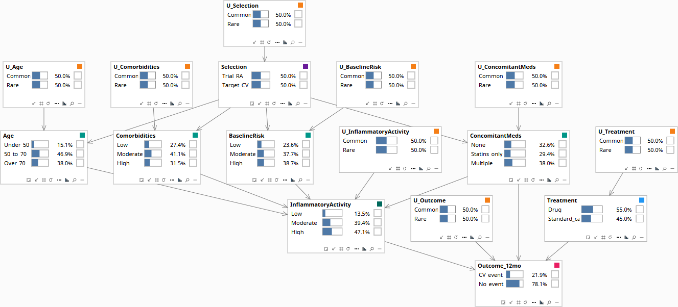
The model adds an explicit selection node S — labeled Selection in the diagrams below, marked by a small purple rectangle in its title bar to distinguish it from confounders, decisions, outcomes, and U-nodes. S indicates which population the patient is drawn from. Edges from S to other nodes encode the dimensions along which the populations differ.
| Node | States | Role |
|---|---|---|
| S (selection) | Trial_RA · Target_CV | Population indicator |
| Age | Under_50 · 50_to_70 · Over_70 | Differs across populations |
| BaselineRisk | Low · Moderate · High | CV-event-specific risk score; differs across populations |
| Comorbidities | Low · Moderate · High | Differs across populations |
| ConcomitantMeds | None · Statins_only · Multiple | Differs across populations |
| InflammatoryActivity | Low · Moderate · High | The shared mechanism — same effect in both populations |
| Treatment | Drug · Standard_care | Decision |
| Outcome_12mo | CV_event · No_event | Target outcome |
Edges: S → Age, BaselineRisk, Comorbidities, ConcomitantMeds (population-level distributional shifts). All four → InflammatoryActivity (the shared mechanism mediates upstream effects). InflammatoryActivity, ConcomitantMeds, Treatment → Outcome_12mo.
Critically, the diagram has no direct edge from S to InflammatoryActivity or Outcome_12mo — visible in the screenshots below by tracing arrows out of the purple-marked Selection node and noting that they reach only the four covariates, never the mechanism or the outcome. Those absences are the formal transport assumption. They say: once you condition on the demographic and clinical covariates that selection depends on, the mechanism and the outcome are exchangeable across populations.
Under the transport DAG above, P(Outcome | do(Treatment), S = Target_CV) is identifiable. The recipe is: estimate P(Outcome | do(Treatment), covariates, S = Trial_RA) from the trial data; reweight by the target population's distribution of covariates. This is the formal version of "post-trial reweighting." It works only because the diagram excludes a direct effect of S on the mechanism. If that exclusion is wrong — if the trial selected on a mechanism-relevant feature not measured — the reweighted estimate is biased, and the bias is not detectable from trial data alone.
The Three Queries
The transport diagram supports three queries with three distinct identification strategies.
How to read the diagrams. An arrow shows the causal direction. An arrow from A to B means A causes an effect — a change — in B.
Two operators appear repeatedly below. obs(X = value) means we learned that X had this value — like filtering the chart-review down to only patients where X was that value. do(X = value) means we imposed this value — like a randomization in a trial, where we control X regardless of what the patient would naturally have. The difference matters: filtering down to "patients who got the drug" tells you something about which patients tend to receive it; imposing the drug tells you only what the drug does.
What was the survival curve for drug-treated patients in the RA trial?
P(Outcome_12mo | Treatment = Drug, Selection = Trial_RA). Read directly from the trial data, conditional on Age, BaselineRisk, Comorbidities, and ConcomitantMeds as observed in the trial. Applies only to the trial population.

Population baseline before any patient data is entered. All nodes at their marginal prior distributions.
What would the CV event rate be in the target population if we deployed the drug?
P(Outcome_12mo | do(Treatment = Drug), Selection = Target_CV). Identifiable under the transport assumptions encoded in the DAG: estimate the conditional treatment effect within the Trial_RA arm; reweight to the Target_CV population's covariate distribution over Age, BaselineRisk, and Comorbidities. Whether this is the right answer depends on whether the no-direct-effect-of-S assumptions hold — a domain-knowledge question the DAG forces explicit.

Population baseline. Selection is at its prior.
For this specific CV patient with their specific covariate profile, what is the expected treatment-effect contrast?
Three operations on the same graph: (1) Set the patient's observed covariates — Age, BaselineRisk, Comorbidities, and ConcomitantMeds — with Selection set to Target_CV. Abduction updates the patient's U-values away from the population priors, capturing what the covariates and population indicator imply about this person's idiosyncratic biology. (2) Compute the contrast: do(Treatment = Drug) versus do(Treatment = Standard_care), each evaluated under the abducted U-values. (3) Read the difference. The output is a posterior distribution over the treatment effect for this individual — not the population average — plus an e-value quantifying how strong an unmeasured selection mechanism would have to be to overturn the recommendation.
Population baseline before any patient data is entered.
Download the Model
The Bayes Server file below encodes the DAG and the conditional probability tables described above. Each observable node has a corresponding U-node — the exogenous noise variable that absorbs residual variation — which is what makes Rung 3 counterfactual abduction possible. The CPTs are populated with clinically defensible illustrative priors; the qualitative behavior they encode is what makes the failure mode visible when running Rung 1 versus Rung 2 queries on the same data.