Identification is a property of the graph, not the data.

The identification problem

A randomised controlled trial solves the identification problem by construction: random assignment to treatment breaks the correlation between treatment and confounders, so the observed difference in outcomes is entirely attributable to the treatment. Most real decisions cannot wait for an RCT — the treatment has already been applied, the experiment is too expensive, or randomisation is unethical.

The question becomes: under what conditions can we estimate the causal effect P(Y | do(X=x)) — the distribution of Y if we were to forcibly set X to x — from observational data where we only have access to P(Y | X=x) — the distribution of Y among those who happened to have X=x?

The answer depends entirely on the causal graph. The same observational data supports identification under one graph and fails under another. Without the graph, you cannot know whether your estimate is valid — even asymptotically, with infinite data.

The back-door criterion

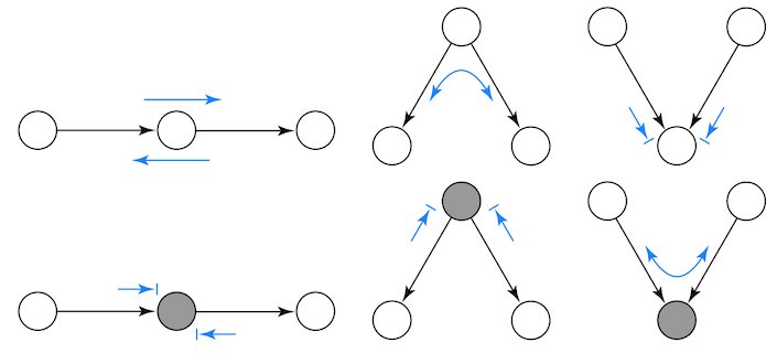
A set of variables Z satisfies the back-door criterion relative to an ordered pair (X, Y) in a DAG G if: (1) no variable in Z is a descendant of X; and (2) Z blocks every path between X and Y that contains an arrow into X (a “back-door path”).

If Z satisfies the back-door criterion, then the causal effect of X on Y is identified and equal to:

P(Y=y | do(X=x)) = ∑_z P(Y=y | X=x, Z=z) P(Z=z)

This is the adjustment formula. It says: stratify by Z, compute the conditional probability of Y given X and each stratum of Z, and average over the population distribution of Z. This is what a regression “controlling for Z” is attempting to compute — but only works causally when Z satisfies the back-door criterion, which cannot be verified without the graph.

The front-door criterion

Consider the canonical case: X → M → Y, with an unobserved confounder U affecting both X and Y. The back-door criterion fails because U is unobserved and cannot be adjusted for. But the front-door criterion may still identify the causal effect if: (1) M is the only path from X to Y; (2) there are no unobserved confounders between X and M; and (3) all back-door paths from M to Y are blocked by X.

The front-door adjustment formula computes the causal effect in two steps: first estimate the causal effect of X on M (which is identified because there are no unobserved confounders on that path); then estimate the causal effect of M on Y adjusting for X (which blocks the back-door path through U). The composition of these two effects gives the total causal effect of X on Y.

The canonical example: estimating the effect of smoking on lung cancer when unobserved genetic factors affect both smoking propensity and cancer risk. If tar deposits in the lungs are the only causal pathway, and tar can be measured, the front-door criterion applies. The historical significance: this was the example Pearl used to show that causal effects can be identified even in the presence of unobserved confounding, provided the causal graph has the right structure.

Do-calculus

Do-calculus is a system of three inference rules for transforming expressions involving the do-operator into expressions that can be computed from observational data. The rules govern when it is valid to: (1) add or remove an observation; (2) exchange an observation for an intervention; or (3) exchange an intervention for an observation.

The back-door and front-door criteria are special cases — they apply when a single application of a standard adjustment is sufficient. Do-calculus handles the general case, including complex graphs where identification requires a sequence of transformations. Pearl proved that do-calculus is complete: a causal effect is identifiable if and only if do-calculus can derive a formula for it in terms of observational distributions.

For most practical enterprise risk applications, the back-door criterion is sufficient. Do-calculus becomes necessary when the causal graph has complex structure — multiple unobserved confounders, selection bias, or measurements made under different experimental regimes. The key practical implication is that identifiability is a property of the graph, not the data — and the graph must be specified before the question of identification can even be posed.

When identification fails

Identification fails when there is an unobserved confounder on a path that cannot be blocked by any combination of observed variables, and the front-door criterion also fails (because the mediating pathway is also confounded or not fully measured). In these cases, the causal effect cannot be uniquely determined from observational data — any estimate is a function of untestable assumptions about the distribution of the unobserved confounder.

The honest response to non-identification is sensitivity analysis: specify the range of plausible values for the unobserved confounding, and compute how the causal effect estimate changes across that range. If the conclusion is robust to the full plausible range, proceed. If the conclusion reverses within the plausible range, the observational data alone is insufficient and a design-based approach — an instrument, a natural experiment, a discontinuity — is required.

The key point for risk practitioners: declaring a causal effect “estimated” when identification has not been established is not a conservative error. It is precisely wrong in a direction that depends on the sign of the omitted confounding — which may be exactly the direction that leads to the worst decision.