Why a Causal Model
A clinician reviewing an elevated LDL of 145 mg/dL faces a standard question: is this patient's cardiovascular risk adequately managed? The standard answer is to titrate the statin until LDL falls to target. But the model encodes a different question first: why is the LDL elevated? If the patient is also on medications known to cause weight gain and dyslipidemia—antipsychotics, corticosteroids, antiretrovirals, certain antiepileptics—then a substantial share of the observed BMI and LDL may be iatrogenic. The statin is not managing the patient's underlying lipid biology; it is partially compensating for a drug-induced elevation. A standard regression cannot separate these two contributions because it treats observed LDL as a single fact about the patient. The causal model encodes the path from Medications through BMI to LDL, and separately from Medications directly to LDL, as structural relationships. Holding the patient's biological background fixed through the exogenous nodes, it can change one input—the medication—and read the counterfactual output. The difference between the observed LDL and the counterfactual LDL is the iatrogenic contribution. That number is what the prescribing decision is actually responsible for.
| Analysis Component | Standard Approach | Causal Approach |
|---|---|---|
| Medication–BMI relationship | BMI treated as a patient characteristic; medication use included as a covariate at most | Direct causal path from Medications to BMI encoded in the graph structure |
| LDL attribution | Observed LDL assigned entirely to patient-level risk factors | LDL decomposed into underlying biology, BMI-mediated, and direct medication-induced components |
| Statin dosing adequacy | Statin dose assessed against the observed (partly iatrogenic) LDL | Statin dose assessed against the counterfactual LDL the patient would have without the offending medication |
| Hospitalization risk | Confounded: sicker patients receive more medications, so medication effect is entangled with disease severity | do() severs the Medications node from its confounders; the causal effect on hospitalization is isolated |
The Questions
- Given everything true about this patient, what would their BMI, LDL, and hospitalization risk have been without the weight-gaining medications? — Rung 3 (Counterfactual). Answering it requires anchoring the patient's exogenous biological state to their actual history via abduction—holding Age, SocioeconomicStatus, and all U nodes fixed to this specific person—then applying do(Medications=0) and reading the counterfactual outcomes. The confounders Age and SES influence how much medication the patient receives; abduction locks those influences in place so the only thing that changes in the query is the prescription itself.
- If we switch this patient class to a metabolically neutral medication alternative, how much does cardiovascular hospitalization risk fall on average? — Rung 2 (Intervention). A forward-looking do() query that severs Medications from its parents—Age and SocioeconomicStatus—before propagating the effect downstream. Without this severance, the intervention estimate is contaminated by the fact that sicker and older patients tend to receive more of these medications, making the correlation look worse than the true causal effect.
- Given this patient's age and socioeconomic status, what does the model estimate for their baseline metabolic and hospitalization risk before any specific medication history is considered? — Rung 1 (Association). Enters known patient characteristics as observed evidence and reads the updated joint distribution across BMI, LDL, Statins, and hospitalization. At Rung 1 the graph encodes which dependencies exist; inference flows in both directions regardless of arrow direction, and no causal claims attach to the result.
Reading the screenshots: a black check mark on a node means it has been set as observed evidence — a fact entered into the model, acting as a filter. A red check mark means it has been set as a do intervention — a decision applied to the model, severing the influence of its parents.
Reading the spec tables: each Run the Analysis block lists the exact steps to reproduce each screenshot in Bayes Server. The Obs / Do column uses three italic control tokens: clear — reset the model to a blank no-evidence state; abduction step — enter the factual observations that anchor the U nodes to this specific case; use abduction result — apply a do() intervention with the U nodes held from the abduction step.
What the Medication Actually Caused
“Given everything we know about this patient—their age, their socioeconomic situation, their actual BMI and cholesterol readings—what would those numbers have looked like if we had never prescribed the weight-gaining medication?”
Rung 2 gives the average causal effect across patients like this one. Rung 3 asks a sharper question: for this specific patient, given what actually happened, what is the counterfactual? To answer it, the model first runs abduction—entering the patient's observed Age, SocioeconomicStatus, BMI, LDLCholesterol, HospitalizationCV, and Medications as evidence to anchor the exogenous U nodes to this individual's biological background. It then releases the BMI, LDL, and hospitalization nodes (the outcomes are queries, not held observations) and applies do(Medications=0), severing the prescription from all upstream influences and reading the counterfactual distribution. The difference between the abducted state and the counterfactual state is the medication's individual contribution to those outcomes.
Without the weight-gaining medications, this patient's BMI would fall from 61 to 31.8 kg/m²—a reduction of 29 units that the counterfactual attributes almost entirely to the prescription, not the patient's biology. The LDL picture reveals the clinical trap: fully removing medications (do = 0) raises LDL from the observed 100 to 115, because the statin that was prescribed to manage the medication-induced dyslipidemia is also removed. Reducing medications to 5 instead tells a different story—BMI drops to 39.5 and LDL falls to 74.2, because some statin protection remains while the major driver of weight gain is reduced. Non-CV hospitalization risk drops from 1.02 to −9.86 under full removal, and CV hospitalization and mortality both improve in both counterfactual scenarios. The statin is not fighting the disease; it is fighting the other medication—and the model quantifies exactly how much work it is doing.
| Image | Obs / Do | Node | Set to | Result |
|---|---|---|---|---|
| Q1-SLIDE-0 Prior | clear | — | BMI 60.5 ± 1.95 | LDL −36.7 ± 30 | HospNonCV 1.01 ± 1.21 | Mortality −41.8 ± 1.11 | |
| Q1-SLIDE-1 Abduction | clear | — | ||
| obs | Age | 57.2 | ||
| obs | SocioeconomicStatus | 11.9 | ||
| obs | Medications | 18.3 | ||
| obs | BMI | 61 | ||
| obs | LDLCholesterol | 100 | U nodes anchored — HospCV −20.6 | HospNonCV 1.02 | Mortality −41.3 | |
| Q1-SLIDE-2 CF Meds=5 | use abduction result | — | ||
| do | Medications | 5 | BMI 39.5 ± 1.02 | LDL 74.2 ± 28.7 | HospCV −23.9 | HospNonCV −6.95 | Mortality −44.1 | |
| Q1-SLIDE-3 CF Meds=0 | use abduction result | — | ||
| do | Medications | 0 | BMI 31.8 ± 1.02 | LDL 115 ± 28.7 | HospCV −25 | HospNonCV −9.86 | Mortality −45 |

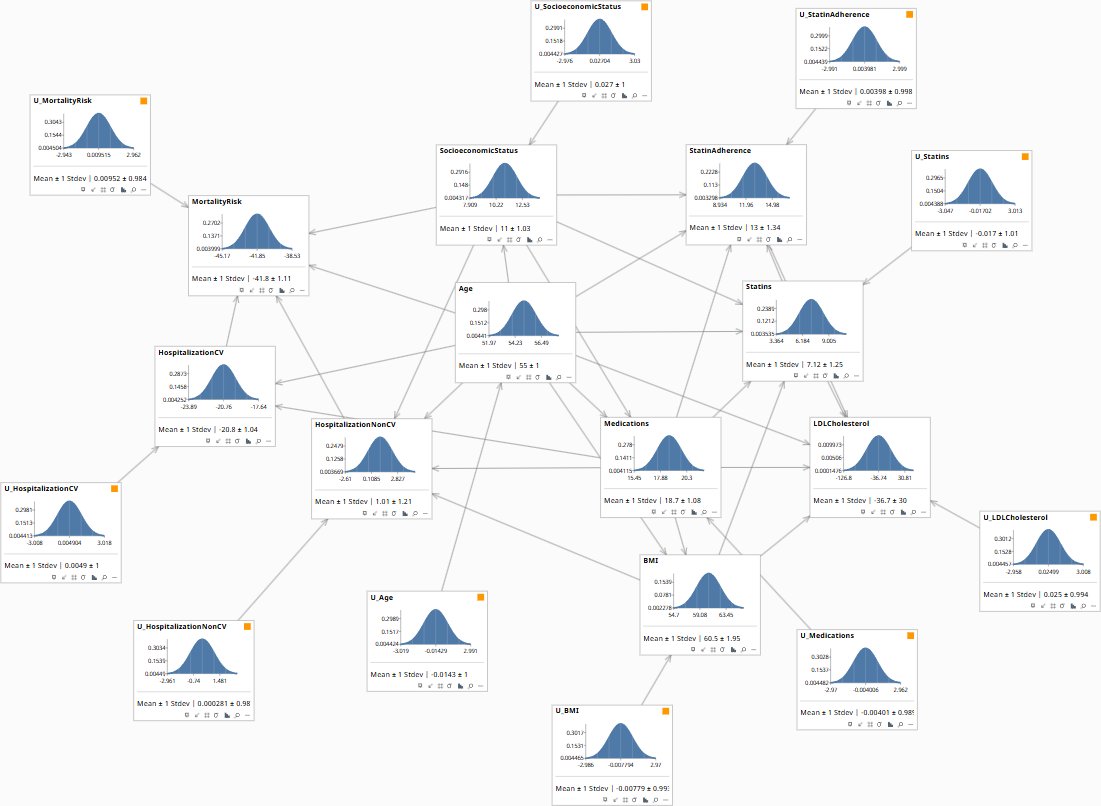
No patient-specific evidence entered. Population marginals: BMI 60.5 ± 1.95, LDL −36.7 ± 30 (model-scale), HospNonCV 1.01 ± 1.21, MortalityRisk −41.8 ± 1.11. These are the reference distributions before any patient data is entered.
What Switching the Medication Class Would Do
“If we move patients on this medication class to a metabolically neutral alternative, what is the actual reduction in cardiovascular hospitalization risk—not the correlation we observe, but the change the switch would cause?”
The observational correlation between Medications and hospitalization is inflated by confounding: older patients and those with lower socioeconomic status tend to receive more of the offending medications and face higher baseline hospitalization risk regardless of the prescription. The model separates these by applying do(Medications=0)—severing Medications from its Age and SES parents before propagating the effect forward. What remains is the pure causal contribution of the medication to hospitalization, stripped of the confounders that make the raw correlation look worse than the true effect. This is the number a prescribing policy should be evaluated against.
The do() intervention on Medications produces a measurable reduction in expected CV and non-CV hospitalization risk, with the hospitalization effect flowing through three concurrent paths: direct (Medications→HospitalizationCV, β ≈ 0.20), BMI-mediated (Medications→BMI→HospitalizationNonCV), and statin-adherence-mediated (Medications→StatinAdherence→LDLCholesterol). Because the do() query severs Age and SES influences on Medications, the estimate is conservative relative to the raw correlation—it removes the portion of apparent risk attributable to the fact that higher-risk patients tend to receive more medications. The reduction in MortalityRisk downstream is the compounded effect through both hospitalization nodes. The policy implication: switching to a metabolically neutral alternative produces a genuine risk reduction, not merely an apparent one driven by patient selection.
| Image | Obs / Do | Node | Set to | Result |
|---|---|---|---|---|
| Q2-SLIDE-0 Prior | clear | — | BMI 60.5 ± 1.95 | HospCV −20.8 ± 1.04 | HospNonCV 1.01 ± 1.21 | Mortality −41.8 ± 1.11 | |
| Q2-SLIDE-1 do(Meds=0.3) | clear | — | ||
| do | Medications | 0.3 | BMI 32.2 ± 1.02 | LDL 112 ± 28.7 | HospCV −24.9 | HospNonCV −9.68 | Mortality −44.9 | |
| Q2-SLIDE-2 do(Meds=0) | clear | — | ||
| do | Medications | 0 | BMI 31.8 ± 1.02 | LDL 115 ± 28.7 | HospCV −25 | HospNonCV −9.86 | Mortality −45 |
No intervention applied. Population prior: HospCV −20.8 ± 1.04, HospNonCV 1.01 ± 1.21, MortalityRisk −41.8 ± 1.11. These are the reference values the do() queries are measured against.
Where This Patient Sits Before the Prescription Is Considered
“Before we look at any medications, what does this patient's age and socioeconomic profile tell us about their expected BMI, cholesterol, and hospitalization risk?”
At Rung 1 the model is running as a filter: enter what is known about the patient, read what updates across the joint distribution. Entering Age and SocioeconomicStatus as observed evidence propagates through the graph's dependency structure—the graph encodes which nodes are genuinely connected to these inputs, so only the nodes with a conditional dependence on Age or SES update. The result is a patient-specific prior: where this person sits on the BMI, LDL, Medications, Statins, and hospitalization distributions before any clinical details are entered. This is the baseline the Rung 2 and Rung 3 queries are measured against.
Entering Age=62 alone shifts expected medications upward to 21, BMI to 64.5, and worsens mortality risk to −39.5 — but adding SES=−0.8 reverses the BMI gain while further worsening mortality to −37.2. That counterintuitive result is the adherence pathway made visible: lower SES knocks StatinAdherence from 15.9 down to 9.79, which reduces statin coverage and lets LDL drift upward from −108 to +36 (model-scale). The mortality penalty from reduced adherence outweighs the modest BMI benefit from lower socioeconomic-driven medication load. At Rung 1 none of these updates carry causal meaning — the graph encodes which dependencies exist, and inference flows both ways regardless of arrow direction. The clinical value is orientation: a 62-year-old with low SES carries compounding risk through the adherence channel that a BMI reading alone would understate.
| Image | Obs / Do | Node | Set to | Result |
|---|---|---|---|---|
| Q3-SLIDE-0 Prior | clear | — | Age 55 ± 1 | Meds 18.7 ± 1.08 | BMI 60.5 ± 1.95 | HospNonCV 1.01 ± 1.21 | Mortality −41.8 ± 1.11 | |
| Q3-SLIDE-1 obs(Age=62) | clear | — | ||
| obs | Age | 62 | Meds ↑ 21 ± 1.03 | BMI ↑ 64.5 ± 1.86 | HospCV −19.6 | HospNonCV 2.8 | Mortality −39.5 | |
| Q3-SLIDE-2 obs(Age=62, SES=−0.8) | clear | — | ||
| obs | Age | 62 | ||
| obs | SocioeconomicStatus | −0.8 | Meds 18 ± 1 | BMI 60.1 ± 1.83 | StatinAdh ↓ 9.79 | HospNonCV ↑ 3.19 | Mortality −37.2 |

Population baseline before any patient characteristics are entered. Age 55 ± 1, Medications 18.7 ± 1.08, BMI 60.5 ± 1.95, HospNonCV 1.01 ± 1.21, MortalityRisk −41.8 ± 1.11. Enter age and SES to orient the patient on the joint distribution.
Try the Model
Download the Models
* This is a hypothetical model constructed for illustration purposes only. Variable distributions, coefficients, and causal structure are representative rather than clinically validated. It is not intended for use in clinical decision-making.
All models require Bayes Server (free edition available). See Download Models for the full library.
If your patients are on medications with known metabolic side effects, your current risk models are attributing drug-induced BMI and LDL elevation to the patient's biology—overstating their baseline risk and potentially over-treating with statins a problem that a prescription change could address directly.
The models are free. What I provide is the judgment to build the right structure for your specific patient population, encode your clinicians’ knowledge into it, and turn the output into treatment decisions that distinguish what the disease is doing from what the medication is doing. The discipline stays with your team.