Why a Causal Model
Pharmacoepidemiology has a well-developed Rung 2 toolkit. Cohort studies, case-control studies, self-controlled case series, target-trial emulation — these all answer the population-level question: across many patients, how does drug exposure shift the distribution of an adverse outcome? That is sufficient for regulatory approval and for population-level risk-benefit analysis.
It is not sufficient for the individual question that drug-injury cases, M&M conferences, and causality-assessment frameworks (WHO-UMC, Naranjo, RUCAM) actually ask: in this specific patient, with this specific exposure, did the drug cause the injury? That is a Rung 3 counterfactual claim — and answering it requires structural commitments that go beyond what a Bayesian network can offer on its own.
A standard Bayesian network can compute P(AKI | NSAID, covariates) at Rung 1 and P(AKI | do(NSAID), covariates) at Rung 2. It cannot, by itself, compute P(AKI = No | do(NSAID = No), this patient's observed factual outcome and covariates) — the probability of necessity, the formal version of "but-for cause." That computation requires committing to a structural-equation interpretation of the graph, with explicit exogenous variables that absorb the residual variation. Those exogenous variables — the U-nodes — are abducted from the factual observation, the intervention is applied, and the counterfactual outcome is read.
The Causal Structure
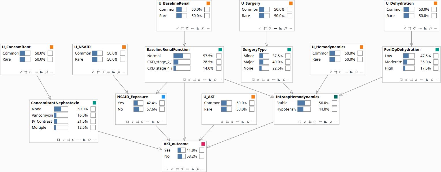
The model is a Structural Causal Model in the strict sense: every endogenous variable has its structural parents AND a corresponding exogenous U-node. The U-nodes are not optional cosmetic additions — they are what makes the counterfactual computation tractable.
| Observable Node | States | Role |
|---|---|---|
| BaselineRenalFunction | Normal · CKD_stage_2_3 · CKD_stage_4_plus | Pre-existing risk |
| SurgeryType | Minor · Major · None | Acute insult |
| PeriOpDehydration | Low · Moderate · High | Modulator |
| ConcomitantNephrotoxin | None · Vancomycin · IV_Contrast · Multiple | Co-cause |
| NSAID_Exposure | Yes · No | Exposure of interest |
| IntraopHemodynamics | Stable · Hypotensive | Mediating variable |
| AKI_outcome | Yes · No | Adverse event of interest |
Each observable also has a U-node — U_NSAID, U_AKI, etc. — modeled as a 2-state exogenous variable with a 50/50 prior. These U-nodes are the residual variation that the structural parents do not explain. They are what an SCM has and a vanilla BN does not.
Edges among observables: BaselineRenalFunction, SurgeryType, PeriOpDehydration → IntraopHemodynamics. IntraopHemodynamics, NSAID_Exposure, ConcomitantNephrotoxin, BaselineRenalFunction → AKI_outcome. (Optionally) BaselineRenalFunction → NSAID_Exposure (CKD reduces NSAID prescribing — confounding by indication in the protective direction).
Rung 2 is identifiable under standard back-door adjustment. Rung 3 — the probability of necessity — is identifiable given the SCM structural assumptions: that the U-nodes are independent across observables, that the structural equations are deterministic given (parents, U), and that the parameterization of those equations is correct. These are testable in some cases (cross-validation against held-out cohorts, comparison to instrumental-variable estimates) and untestable in others. The page-level message: Rung 3 always requires assumptions that go beyond what data alone can support, and naming those assumptions is a precondition for using the inference responsibly in a regulatory or legal context.
The Three Queries
The three queries here are particularly important to distinguish, because they are routinely conflated in pharmacovigilance practice. Each panel below is a screenshot of the actual Bayes Server model — click a button to step through the slides.
How to read the diagrams. An arrow shows the causal direction. An arrow from A to B means A causes an effect — a change — in B.
Two operators appear repeatedly below. obs(X = value) means we learned that X had this value — like filtering the chart-review down to only patients where X was that value. do(X = value) means we imposed this value — like a randomization in a trial, where we control X regardless of what the patient would naturally have. The difference matters: filtering down to "patients who got the drug" tells you something about which patients tend to receive it; imposing the drug tells you only what the drug does.
Among patients with this covariate profile who took the NSAID, what fraction developed AKI?
Read directly from the data as a conditional probability. As covariates accumulate, the AKI rate climbs — but watch P(NSAID = Yes) drop in the first slide. Clinicians prescribe NSAID_Exposure less in patients with CKD stage 2-3, precisely because they fear AKI. The covariate is informative about both the outcome AND the prescribing decision; the conditional cannot tell you which is which.

Population baseline before any patient data is entered. AKI, NSAID exposure, and the covariates all sit at their marginal priors.
If we forced NSAID exposure on a random patient — without conditioning on the prescribing rule — what would the AKI rate be?
The do-operator severs the BaselineRenalFunction → NSAID_Exposure edge, breaking the back-door from CKD into the prescribing rule. What remains is the unconfounded population-level effect of the NSAID on AKI_outcome. This is the standard regulatory question — sufficient for label warnings and prescribing guidelines.
Population baseline. NSAID is at its prior — some patients exposed, most not, driven by the natural prescribing rule that depends on renal status.
This patient took the NSAID and developed AKI. Would the AKI have occurred if they had not taken the NSAID?
Three operations on the same graph: (1) Set the patient's full evidence — BaselineRenalFunction = CKD_stage_2_3, SurgeryType = Major, PeriOpDehydration = Moderate, ConcomitantNephrotoxin = None, IntraopHemodynamics = Hypotensive, NSAID_Exposure = Yes, AKI_outcome = Yes. The U_AKI posterior shifts away from 50/50 — that's the abduction step, encoding this patient's idiosyncratic AKI susceptibility. (2) Carry the abducted U_AKI forward as soft evidence. (3) Apply do(NSAID_Exposure = No) to read the counterfactual outcome.

Population baseline before any patient data is entered. All nodes at their marginal priors.
Download the Model
The Bayes Server file below encodes the DAG and the conditional probability tables described above. Each observable node has a corresponding U-node — the exogenous noise variable that absorbs residual variation — which is what makes Rung 3 counterfactual abduction possible. The CPTs are populated with clinically defensible illustrative priors; the qualitative behavior they encode is what makes the failure mode visible when running Rung 1 versus Rung 2 queries on the same data.