How the reserve number got built.

The starting question

The reserve committee meets quarterly. The chief actuary presents the chain-ladder development factors, the Bornhuetter-Ferguson estimate, and the reserve range. For most of the prior decade the chain-ladder triangle was a clean predictor — the development pattern was stable enough that the loss development factors (LDFs) at each maturity gave a defensible point estimate, and the BF estimate served as a sanity check tied to expected loss ratios. Reserve adequacy was “within the range.”

By Q2 2023 that had stopped working. The 12-to-24-month and 24-to-36-month development factors were drifting upward. The drift was not uniform across accident years: 2019 looked nearly normal at 48 months of maturity; 2020 was anomalous in the way COVID years were anomalous everywhere; 2021 was developing adversely at a pace that did not match either 2019 or 2020; 2022 was incomplete but tracking worse than 2021 at the same maturity.

The chief actuary’s position going into the engagement: “Chain-ladder is telling us the pattern is shifting. It is not telling us why. We can extrapolate the shift, but that extrapolation assumes the cause of the shift continues at the same rate, and we have no basis for that assumption.” The reserve committee wanted a structural account before approving the reserve, because the auditor was going to ask the same question and the regulator was going to ask it later.

In the room for the kickoff: the chief actuary, the head of commercial claims, the chief data officer, the head of underwriting for commercial auto, and outside counsel (briefly, for the legal-environment context). The engagement was eight weeks. Half-day audit at week one; model construction across weeks two through six; validation at week seven; presentation to the reserve committee at week eight.

What the data showed

Standard insurance reserving data: incremental and cumulative paid-loss triangles by accident year and development maturity, case reserves at each diagonal, allocated and unallocated loss adjustment expenses (ALAE and ULAE), reported claim counts, average severity by quarter of development, and a small set of supplementary indicators — attorney-represented case rate, average time-to-settlement for litigated claims, share of claims with a third-party liability component above a $250K threshold.

The chain-ladder triangle, plotted, showed three things:

• Pre-2019 accident years: stable LDFs. Pattern matched a long-term industry pattern for commercial auto BI (bodily injury).
• 2019–2020: 2019 LDFs slightly elevated; 2020 LDFs anomalous due to traffic-volume collapse and court closures. Not a useful signal.
• 2021–2023: LDFs systematically elevated. The 24-to-36 development factor for AY 2021 was running ~12% above the ten-year average. AY 2022 at the same maturity was running ~16% above. AY 2023 incomplete but on a similar trajectory.

The supplementary indicators showed the most useful signal: the attorney-represented case rate had risen from 22% of cases pre-2019 to 38% of cases for AY 2022. Average time-to-settlement for litigated claims had risen from 21 months to 33 months. The share of claims above the $250K third-party threshold had grown from 8% to 14%.

The chain-ladder triangle is blind to these indicators. It sees only the paid and case-reserve numbers on the diagonal. The supplementary indicators say the case mix is shifting — the structural composition of claims is different, not just the development speed. That is the question chain-ladder cannot answer.

First model attempt — and what it missed

The first model the team built was a structural causal model with the following nodes:

• Accident year (AY) as the contextual root.
• Underlying claim frequency and underlying severity as latent drivers.
• Reporting lag from accident to claim open.
• Settlement lag from claim open to closure.
• Paid losses at each development maturity as observed outputs.

The DAG was clean. It encoded the basic mechanics of how losses develop. Fit against the pre-2019 data was excellent — the model reproduced the historical chain-ladder pattern almost exactly, because the structure encoded the same logic chain-ladder encodes implicitly.

Fit against the 2021–2022 data was bad. The model was systematically under-predicting paid losses at 24 and 36 months of maturity. The team had built a structural account of the prior decade’s reserving process. It was as blind to the post-2020 shift as chain-ladder was.

The diagnostic conversation in that week: what is the model missing? The model represented the loss development process correctly. The error meant something in the world was driving losses through a path the model didn’t represent.

The head of commercial claims raised the point that ended up restructuring the model: “The claims that are settling in 2022 don’t look like the claims that settled in 2018. The mix is different. The same accident severity now resolves through a different process — more attorney involvement, more time in litigation, more pressure to settle above policy limits. The development factor is high because the case is being processed differently, not because the underlying loss is different.”

That is a structural claim, not a parametric one. It says there is a node missing from the DAG — something like “case handling regime” or “litigation environment” — that mediates between the underlying loss and the paid amount. The first model had no such node.

The expert sessions

Three sessions, each ninety minutes. The framing for each was the same: name the things that affect a claim’s development that are not already in the model. Not opinions on reserve levels. Mechanism.

Session one — commercial claims. The head of claims described three structural changes since 2018: (a) plaintiffs’ firms had moved more aggressively into commercial auto in this region; (b) the local court system had become noticeably more plaintiff-friendly in jury awards following two specific appellate decisions in 2020 and 2021; (c) the company’s own claims-handling protocol had shifted in late 2019 toward earlier and more proactive engagement with represented claimants. The first two pushed paid losses up. The third was intended to reduce litigation costs but, in practice, settled more cases at higher amounts.

Session two — underwriting. The head of underwriting described two changes in the book of business itself: (a) growth in the long-haul trucking segment over 2019–2021 (a higher-severity segment than light commercial); (b) tightening of underwriting standards in late 2021 to slow that growth. The composition of the book at the time of each accident year mattered. Mix shift was not constant.

Session three — outside counsel. Confirmed the two appellate decisions and added a third pending case at the state supreme court that could materially affect the legal environment going forward. Provided a rough estimate of the directional effect of each decision on settlement values, with explicit uncertainty.

The structural drivers identified across the three sessions:

• Legal environment — appellate-decision-driven, time-varying by region and by year.
• Case handling regime — the insurer’s own claims protocol; changed in late 2019.
• Book composition — long-haul vs light commercial mix; changed across the period.
• Plaintiff bar activity — correlated to but distinct from the legal environment.

The DAG was redrawn. Each of these became a node. Legal environment, case handling regime, and plaintiff bar activity all influence a new intermediate node, case settlement multiplier, which sits between underlying loss and paid amount. Book composition influences underlying severity. Accident year becomes a context variable that constrains all of these — the legal environment in 2018 is different from the legal environment in 2022 in ways the model can now represent.

Where the experts disagreed

Two specific disagreements surfaced and had to be reconciled, not papered over.

Disagreement one: the dominant driver of the post-2020 LDF drift. The chief actuary’s prior was that the drift was primarily a social inflation phenomenon — a broad legal-environment shift, applicable to most cases in the book. The head of claims’ prior was that the drift was concentrated in attorney-represented cases, a specific case-mix shift, with the underlying non-litigated cases developing normally. Both were partially right and the difference between their two stories implied different futures: if the actuary was right, the trend continues across the whole book; if the claims VP was right, the trend stabilises once attorney-representation rates plateau.

The data could in principle resolve this if it were stratified. The team pulled the paid-loss triangles separately for attorney-represented and non-represented claims for AYs 2018–2022. The result: non-represented claims developed within historical norms. The drift was concentrated in attorney-represented cases, but the share of attorney-represented cases was itself increasing, and the development pattern of attorney-represented cases was also shifting. Both effects were real; neither story alone was sufficient.

The model needed both. Attorney representation became its own node, with two paths to paid loss: a path through case selection (which cases get represented) and a path through development behavior (how represented cases settle).

Disagreement two: the magnitude of the 2020 appellate decision’s effect. Outside counsel estimated the decision had increased settlement values by 8–15% for cases in its jurisdiction. The chief actuary’s read of the data suggested the effect was closer to 3–7% on average across the book (because the decision applied to only one of the twelve states). The head of claims’ experience suggested a higher number for cases that actually went to verdict, lower for those that settled early in negotiation.

The three estimates were not contradictory; they were estimates of different conditional quantities. Counsel was estimating the effect on jurisdiction-affected cases at verdict. The chief actuary was estimating the book-average effect. The head of claims was distinguishing settled-early from late-verdict cases. The reconciliation was structural: the model now needed a path from appellate-decision exposure (a function of accident year and state) through case-route within the legal process (early settlement vs late verdict) to the case settlement multiplier. Each expert was estimating one piece of that path.

Reconciliation

Once the structural disagreements were resolved by adding nodes — rather than by averaging the experts’ numerical estimates — the parameter elicitation became more constrained. Each expert was asked for estimates of the specific conditional quantity the structure now identified them as the authority on. The chief actuary parameterised the base loss-development distributions; the head of claims parameterised the conditional distributions for represented vs non-represented cases; outside counsel parameterised the legal-environment shift conditional on jurisdiction.

Where two experts had overlapping authority on the same conditional, their estimates were combined formally rather than averaged informally. The technique was Bayesian reconciliation of expert priors, with stated variance on each estimate. The full method is documented at Reconciling Expert Parameters; the worked example there uses the same machinery this engagement used.

The output of the reconciliation phase was a parameterised DAG: every node had a distribution, every distribution had stated variance, every variance reflected one or more named experts’ calibrated uncertainty rather than a default flat prior.

The model itself

What the parameterised DAG looked like at the end of week six. Six nodes, seven edges. Injury Severity and Legal Environment are the contextual roots. Legal Representation sits between them and Settlement Value, with both a selection path (which cases get represented) and a behavior path (how represented cases settle). Claims Management Quality mediates between the carrier’s claims protocol and Ultimate Loss. The edge from Injury Severity to Claims Management Quality is the back-door confounder named in the diagnostic phase: carriers with more severe injury mixes invest more heavily in claims management for reasons that are also correlated with ultimate loss. An intervention on Claims Management Quality — do(CMQ=High) — severs this edge, exposing the causal effect separately from the selection effect.

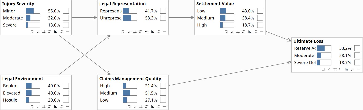
The Claim Development model in Bayes Server — prior distributions on every node, before any evidence is set. Click to enlarge.

The model in Bayes Server format is available below. It loads in Bayes Server natively; the same XML structure is readable by any compliant Bayesian-network tool. The insurer’s data science team chose pgmpy for production inference; the model loads there with a standard XML parser.

The construction-phase narrative above named additional structural elements — case handling regime, plaintiff bar activity, book composition, appellate-decision exposure — that the final model represents through this six-node abstraction. Case handling regime is captured by Claims Management Quality. Plaintiff bar activity is folded into Legal Environment (its operational signal at the modeling scope). Book composition acts through Injury Severity (the long-haul mix shifts the prior distribution of severity). Appellate-decision exposure acts through Legal Environment (jurisdiction-conditional). The narrative talks about the structural drivers as the experts named them; the model captures them at the level of resolution actually identifiable from the data. The compression is part of the discipline.

Validation against prior years

The model was fit on AYs 2018 and prior (treated as “training”) and tested against AYs 2019–2021 (treated as holdout). For each holdout year, the model produced an ultimate-loss distribution; that distribution was compared to the now-observed actual development.

Three results worth naming:

• AY 2019: model’s point estimate was 1.4% above ultimate, within the model’s 50% credible interval. Acceptable.
• AY 2020: model under-predicted by 6%, just outside the 80% credible interval. The miss was traced to the COVID-period claim-volume collapse interacting with the case-handling-regime change; the model represented one but not the other. This pointed at a residual issue with the case-handling-regime node, which was refined accordingly.
• AY 2021: model’s point estimate was within 2% of the maturity-adjusted ultimate. The new structural account of the post-2020 shift was holding up.

The 2020 miss was the most useful result. It told the team that the case-handling-regime node was still imperfect and gave a directional refinement to make. The refined model was then re-validated against 2020 and the residual was reduced to within the credible interval.

Sensitivity analysis showed which parameters drove which outputs. The two parameters with the largest leverage on the AY 2022–2023 reserve point estimate were (a) the conditional probability of attorney representation given accident severity, and (b) the legal-environment shift magnitude. The reserve committee paid particular attention to these two as candidates for ongoing monitoring.

The answer the model gave

The reserve committee’s question was: what is the ultimate-loss estimate for accident years 2019 through 2023, and how confident are we?

The model’s answer for AYs 2019–2023, summed:

• Point estimate: 11.4% above the chain-ladder estimate. The dollar value is omitted here because the engagement is anonymised; the directional finding is the relevant part.
• 50% credible interval: 8.8% to 14.1% above chain-ladder.
• 80% credible interval: 6.2% to 17.0% above chain-ladder.

The structural account behind the number: the elevated development was driven primarily by a case-mix shift (more attorney-represented cases) interacting with a legal-environment shift (higher settlement values per attorney-represented case in two of twelve states). Both effects were partially offsetting against an improving book composition (the late-2021 underwriting tightening had reduced exposure in the higher-severity long-haul segment). Net: reserves needed to increase, but by less than a naive extrapolation of the LDF drift would have suggested.

The reserve committee approved a reserve at the model’s point estimate plus a margin sized to the 80% credible interval’s upper bound. The auditor accepted the structural account in supporting documentation; the regulator’s subsequent inquiry was answered with the same account.

What survived after the engagement

What the insurer kept after week eight:

• The model file in interchange format. Runnable from open-source tools (their data science team chose pgmpy; they were Python-native).
• The elicitation record — which expert provided which parameter, with what stated uncertainty, in which session.
• The validation cases (AYs 2019–2021) as a regression-test suite.
• The sensitivity analysis as a baseline.
• A quarterly refinement cadence: at each reserve review, the chief actuary’s team would re-estimate the two highest-leverage parameters (attorney-representation conditional, legal-environment shift) using the prior quarter’s development. The model itself was retained; the parameters were updated.

The insurer ran the model for three subsequent quarterly cycles without my involvement. At the fourth cycle, they added a new node (a regulatory change affecting commercial auto rate filings in one state) themselves, using the same elicitation protocol the engagement had established. That is the day-2 maintenance picture working as designed.

Day-2 events the team handled themselves

Illustrative day-2 events of the kind a maintained model surfaces. The examples are representative of what happens when a causal model is genuinely owned by the team running it — not all happened in this engagement, but each is the pattern the maintenance practice is designed to support.

• Quarter 2 — an unexpected attorney-representation shift in one state. The quarterly re-estimation showed attorney-rep rates jumping from 42% to 51% in a single state over one quarter. The team checked the sensitivity-analysis baseline: this parameter was one of the two highest-leverage drivers. They ran the model conditional on the new rate and surfaced the implied reserve revision to the reserve committee at the next meeting — before the development data on the affected accident years had matured enough for chain-ladder to detect anything.
• Quarter 3 — a validation-case regression after a parameter refinement. The team refined the legal-environment node based on a third appellate decision. Running the regression-test suite, the model now predicted AY 2020 outside the 50% credible interval again — a worse fit than before the refinement. They traced the regression: the new legal-environment parameter was too aggressive, pulling other accident years off their validated targets. They walked back the parameter and re-validated. Caught before the refinement reached the reserve committee.
• Quarter 4 — a new node added independently. A state-level regulatory change affected commercial auto rate filings in one of the twelve states. The chief actuary’s team identified that the change affected the relationship between book composition and severity in that state, but not in others. They added regulatory-environment-by-state as a new node with one parent (state) and an edge to severity, using the same elicitation protocol the engagement had established. The model file gained one node; the elicitation record gained one session. The validation suite was extended with a holdout case for the affected state.
• Year 1 review — one parameter fell out of its expected range. The annual review compared the prior year’s sensitivity-analysis baseline against the current parameter values. The conditional probability of severe injury given long-haul exposure had drifted upward by 12% — outside the noise band. Diagnostic conversation with the head of underwriting surfaced a change in the trucking-segment mix the underwriting team had been tracking informally but had not yet flagged operationally. The drift was real; the model was the first place it became visible as a structural parameter rather than as anecdotal claim severity.

Each of these events is a normal day in the life of a maintained causal model. The model is not a one-time deliverable that sits on a shelf; it is an artifact that gets used quarterly, refined when evidence shifts, and extended when the world changes in ways the original structure did not anticipate. The team that runs it learns the practice of running it.

What this page is for

This is a construction walkthrough, not a results page. The result is on the case page at executive register. This page exists for the reader — usually a CDO, head of analytics, or technical evaluator — who wants to know what the work actually looks like in eight weeks, with real experts, on a real problem. The answer:

• The first model attempt is usually wrong. The wrongness is informative.
• The expert sessions are where the structural account gets built. The data alone does not contain the structure.
• Where experts disagree, the disagreement points at missing structure, not at parameters to average.
• Validation against prior years is the test the model has to pass before the current year’s answer is trusted.
• What you keep at the end is the model, the elicitation record, the validation cases, and the maintenance practice. The vendor leaves; the artifact and the discipline stay.

For the engagement scope and how the work starts, see The smallest commitment. For the technology and licensing picture, see Stack & Deployment. For the same construction discipline applied in a different domain, see the FAIR cybersecurity risk construction walkthrough.