Almost every observational causal claim rests on a load-bearing assumption: no unmeasured confounding. The estimate is right if there’s no hidden variable doing the work we’re attributing to the treatment. The assumption cannot be tested directly — if it could, you’d measure the variable.
Sensitivity analysis is what honest analysts do instead: quantify how strong an unmeasured confounder would have to be to overturn the conclusion.
The honest problem
An observational study finds that patients on a new drug have 30% lower mortality than patients on standard care, after adjusting for every measured confounder. The headline conclusion: the drug saves lives. The unspoken caveat: conditional on no unmeasured confounding.
What if there is unmeasured confounding? Healthier patients may have been preferentially placed on the new drug. Patients with better insurance get more new drugs and also have better outcomes for unrelated reasons. The unmeasured confounder doesn’t have to be sinister; it just has to exist. The question every reviewer should ask, and most don’t: how strong would such a confounder need to be to fully explain the observed effect?
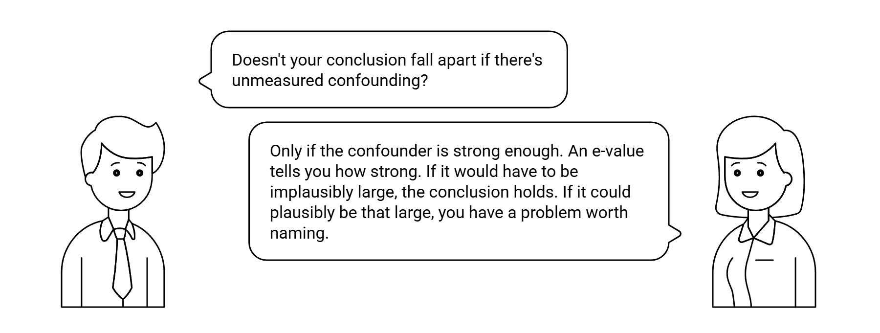
Sensitivity analysis answers exactly that question. Instead of pretending the no-unmeasured-confounding assumption is correct, it computes the strength of the hypothetical confounder required to overturn the result. If the answer is “impossibly strong, much stronger than any known clinical predictor,” the conclusion is robust. If the answer is “about as strong as smoking,” you should worry.
Reviewers sometimes treat sensitivity analysis as a way to undermine results. It is the opposite. A study that survives a stringent sensitivity check is more credible than one that doesn’t. The analyst who computes a high E-value alongside their headline number is announcing “our conclusion is robust to confounders we couldn’t measure.” That is a strength, not a weakness.
The E-value
The simplest, most widely-adopted sensitivity measure is the E-value, due to VanderWeele & Ding (2017).
For a given effect estimate (a risk ratio, hazard ratio, or odds ratio), the E-value is the smallest joint association — on the risk-ratio scale — that an unmeasured confounder would have to have with both the treatment and the outcome to explain away the entire observed effect. Larger E-values mean more robust conclusions.
The formula for a risk ratio RR > 1 is:
An observed RR of 2.0 yields an E-value of 2.0 + sqrt(2.0) = 3.41. To explain that effect away, an unmeasured confounder would have to associate with both treatment and outcome at a risk ratio of at least 3.41 each — stronger than smoking’s association with lung cancer in many populations.
For the lower bound of a confidence interval, you compute a separate E-value answering “how strong a confounder to make the result statistically null?” Both are typically reported.
Cinelli-Hazlett: the linear-regression view
For continuous outcomes and linear regression, Cinelli & Hazlett (2020) developed a sensitivity framework with a different vocabulary but the same goal. They parameterize the strength of an unmeasured confounder by two partial R-squared values: how much of the treatment’s residual variance the confounder explains, and how much of the outcome’s residual variance.
The output is a contour plot showing combinations of those two values that would change the conclusion — usually plotted with reference points marked for measured confounders, so a reviewer can see “to overturn this result, you’d need an unmeasured confounder twice as strong as the strongest measured one.” Concrete and visual; harder to wave away than a single number.
Cinelli-Hazlett works for continuous outcomes; the E-value works for binary or rate outcomes. The two are complementary.
Sensitivity is not robustness
A common misunderstanding: that sensitivity analysis proves the result is correct, or proves the no-unmeasured-confounding assumption holds. It does neither. What it proves is more modest:
- If the assumption is wrong, the unmeasured confounder doing the damage would need to have at least this strength.
- Anything weaker than that, the conclusion holds.
- Anything stronger, the conclusion can be overturned.
The analyst then makes a substantive judgment: is a confounder of that strength plausible in this setting? Domain experts can answer that. The E-value or contour plot is the input to the judgment, not a substitute for it.
When sensitivity analysis is essential
Three settings where sensitivity analysis is not optional:
- Regulatory submissions based on observational data. Real-world evidence, post-market surveillance, comparative effectiveness work. The regulator’s instinct is to assume unmeasured confounding until the analyst proves otherwise. An e-value or sensitivity contour gives the regulator a number to push back against, not a vibe.
- Pharmacovigilance attribution. When a regulator or plaintiff is asking “did the drug cause this adverse event?” based on observational comparisons, the answer is always conditional on unmeasured confounding. The probability of necessity computed in the Pharmacovigilance case study would be paired with a sensitivity analysis in any real submission.
- Risk and policy work where the consequences of being wrong are large. If a wrong conclusion costs lives or millions of dollars, a single point estimate is insufficient. The decision-maker needs to know how much the conclusion can take before it breaks.
Beyond confounding
The sensitivity-analysis idea generalizes beyond unmeasured confounding. The same machinery applies to:
- Selection bias. How strong an unmeasured determinant of selection would need to be to overturn the result?
- Measurement error. How much misclassification of the treatment, outcome, or covariates would change the conclusion?
- Mediation assumptions. A natural direct effect requires an additional, mediation-specific no-unmeasured-confounding assumption. VanderWeele’s framework includes sensitivity analyses targeted at exactly that assumption.
- Transportability. The Drug Repurposing case study’s e-value answers the question “how strong an unmeasured selection mechanism would have to be to overturn the transported recommendation?”
In each case the structure is the same. Specify the strength of an unobserved factor, ask whether the conclusion survives, and report the breaking point. The framework is general; the parameter being varied changes case to case.
The honest version of every observational claim
An observational causal claim with no sensitivity analysis is incomplete. The analyst is implicitly saying “trust me, there’s no unmeasured confounding,” which is exactly what every analyst whose conclusions later turned out wrong was also saying.
The honest version is “our headline estimate is X. To overturn it, an unmeasured confounder would have to have strength Y, which is implausible / plausible / borderline given Z.” The conclusion remains the same; the epistemic status of the conclusion is now visible. A reviewer can argue with the “implausible / plausible / borderline” claim. They cannot argue with the unstated assumption that they don’t even know is being made.
References
Sensitivity analysis has a long history (Cornfield 1959, Rosenbaum 1983), but the modern formulations most useful in practice are the E-value and the Cinelli-Hazlett framework.
The original E-value paper. Defines the metric, derives the closed-form expressions for risk ratios and hazard ratios, and demonstrates the method across published observational studies. Annals of Internal Medicine 167(4): 268–274.
The contour-plot framework for linear regression. Develops the partial-R² parameterization and the “robustness value” summary metric. Journal of the Royal Statistical Society Series B 82(1): 39–67.
The standard reference for matched-pair sensitivity analysis. Develops the Γ parameterization and applies it to a wide range of observational designs. Springer.
Every observational claim should be paired with the e-value or contour plot for the unmeasured confounder that would overturn it. A causal audit names the assumption and quantifies the breaking point.
info@rung3.ai