Why a Causal Model
The clinical observation: among ICU patients with sepsis, those who received vasopressors died at higher rates than those who did not. The naive interpretation: vasopressors are harmful in sepsis. The actual mechanism: clinicians give vasopressors to the patients with worse hemodynamics, and worse hemodynamics independently predict death. The treatment is correlated with the outcome through the prior state, not just through its causal effect.
This is confounding by indication, but it is worse than the static version. The decision is sequential — fluid bolus at hour 0, vasopressor at hour 4, antibiotic escalation at hour 8 — and at each step the patient's evolving state is both an outcome of prior treatment AND a driver of the next treatment decision. Adjusting for the state at each step blocks the legitimate causal pathway from earlier treatment to outcome. Adjusting only for baseline misses the time-varying confounder. Neither standard adjustment strategy works.
Reinforcement learning trained on ICU records learns the historical policy — the policy that produced the observed data. Because the historical policy was driven by the observed state, the policy is a function of the confounder. Deploying a policy learned this way is, formally, a no-op: it reproduces the observed outcomes because it was learned from them. Causal RL — using g-methods or equivalent sequential identification — learns the interventional value of alternative policies, the kind that would produce different outcomes if deployed.

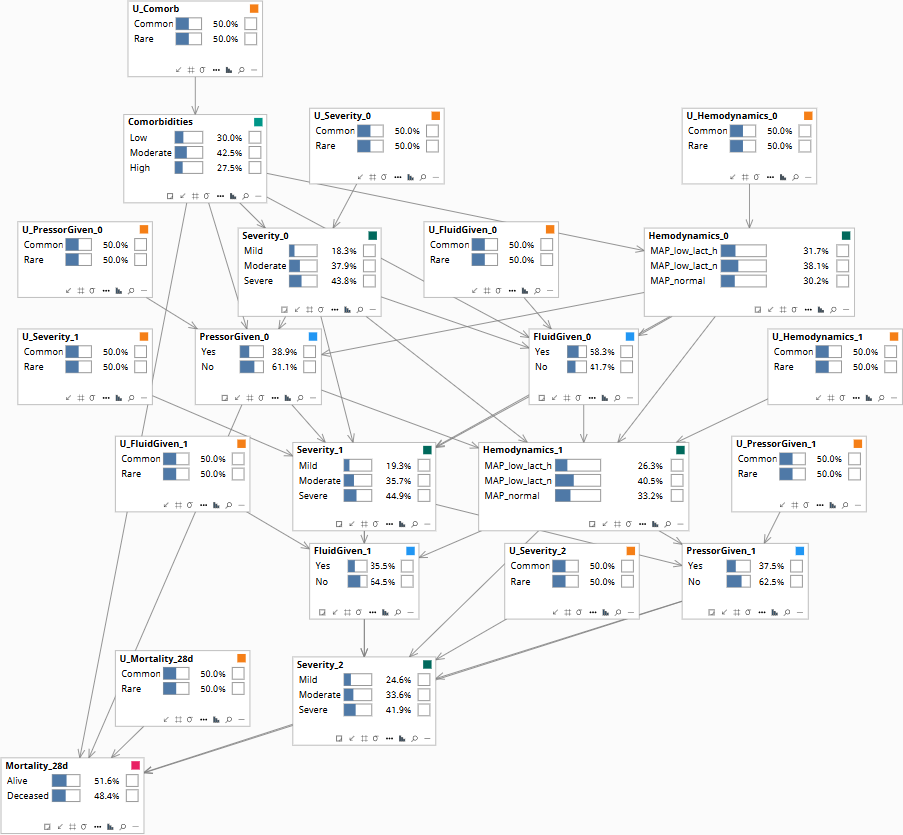
Population baseline before any patient data is entered.
The Causal Structure
The model is a dynamic Bayesian network across three time slices: hour 0 (admission), hour 6, and hour 12. A 28-day mortality node depends on the cumulative trajectory.
| Node (per slice) | States | Role |
|---|---|---|
| Severity_t (SOFA bin) | Mild · Moderate · Severe | Patient state — confounder at next step |
| Hemodynamics_t | MAP_low_lact_high · MAP_low_lact_normal · MAP_normal | Treatment-decision driver — time-varying confounder |
| FluidGiven_t | Yes · No | Treatment |
| PressorGiven_t | Yes · No | Treatment |
| Comorbidities (time-invariant) | Low · Moderate · High | Baseline confounder |
| Mortality_28d (terminal) | Alive · Deceased | Outcome |
The structural commitments at each slice t:
- Severity_t, Hemodynamics_t, Comorbidities → FluidGiven_t, PressorGiven_t (clinicians decide on observed state — the time-varying confounding mechanism)
- Severity_t, FluidGiven_t, PressorGiven_t → Hemodynamics_{t+1}, Severity_{t+1} (treatments and prior state shape next state)
- Final-slice state and cumulative treatments → Mortality_28d
The interventional distribution P(Mortality | do(policy = π̂)) under a candidate dynamic policy π̂ is identifiable using Robins' g-formula: iterate over time slices, taking expectations over the post-treatment state distribution at each step. This is operationally identical to causal reinforcement learning when the value function is computed under the interventional distribution rather than the observational one. The page-level message: the choice between "off-policy RL" and "g-methods" is partly nomenclature; the formal content is identical, and the failure mode of deploying historical policies as causal recommendations is a well-defined statistical artifact.
The Three Queries
Three queries on the dynamic structure, each with a different identification status.
How to read the diagrams. An arrow shows the causal direction. An arrow from A to B means A causes an effect — a change — in B.
Two operators appear repeatedly below. obs(X = value) means we learned that X had this value — like filtering the chart-review down to only patients where X was that value. do(X = value) means we imposed this value — like a randomization in a trial, where we control X regardless of what the patient would naturally have. The difference matters: filtering down to "patients who got the drug" tells you something about which patients tend to receive it; imposing the drug tells you only what the drug does.
Under the historical clinician policy, what fraction of patients with this baseline state survived to day 28?
Computed directly from the joint distribution of Comorbidities, Severity, Hemodynamics, the observed sequence of FluidGiven and PressorGiven decisions, and Mortality_28d. This is what observational survival curves report. Reproduces the data; does not predict the effect of changing clinical practice.
If we deployed an alternative policy — e.g., earlier pressor escalation when MAP drops below 65 — what would the 28-day mortality be?
P(Mortality_28d | do(policy = π̂)). Computed by the g-formula: at each time slice, take the candidate policy's action distribution conditional on the slice's observed Severity and Hemodynamics, and propagate forward through the structural equations. This is the quantity that distinguishes causal RL from off-policy RL with naïve weighting.

Population baseline.
This specific patient received fluid at hour 0 and pressor at hour 12 and died on day 6. Would they have survived if pressor had been started at hour 4?
Patient-specific counterfactual. The U-values at each slice — U_Severity, U_Hemodynamics, U_Mortality — are abducted from the factual observed trajectory; then the intervention do(PressorGiven_1 = Yes) is applied and the trajectory is replayed under the abducted U-values. This is the inference that supports retrospective M&M review and individual-level audit of clinical decisions.
Population baseline before any patient trajectory is entered.
Download the Model
The Bayes Server file below encodes the DAG and the conditional probability tables described above. Each observable node has a corresponding U-node — the exogenous noise variable that absorbs residual variation — which is what makes Rung 3 counterfactual abduction possible. The CPTs are populated with clinically defensible illustrative priors; the qualitative behavior they encode is what makes the failure mode visible when running Rung 1 versus Rung 2 queries on the same data.