The failure mode that Gated Bayesian Networks address is not miscalibration, distribution shift, or Goodhart's Law — though it resembles all three. It is something more specific: a process that has structurally distinct phases, each with genuinely different causal relationships, where a single model is constitutionally incapable of representing both correctly at once. The solution is not a better single model. It is a framework that encodes the phases explicitly and switches between them as evidence accumulates.
The Regime Problem
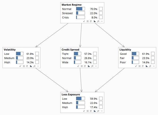
Consider what a credit risk model learns from historical data. During normal credit cycles, the relationship between a borrower's cash flow coverage ratio and their default probability follows a stable conditional distribution. During a liquidity stress event, that relationship changes: borrowers who were perfectly safe under normal conditions become distressed because their refinancing options disappear, not because their underlying cash flows have deteriorated. The causal mechanism is different. The variables that matter are different. The conditional probability tables that were correct last quarter are wrong this quarter.
A single Bayesian network fitted across both periods learns a mixture of the two causal structures. It will not be calibrated correctly in either regime. More importantly, it cannot signal which regime it is currently in — because it has no representation of regime as a concept. It just produces a probability estimate that is an average of what the answer would be in each regime, weighted by their historical frequency.
This is the problem that a Gated Bayesian Network solves. The GBN encodes the regime boundary explicitly:
- Each regime gets its own Bayesian network, calibrated on data from that regime alone
- The boundary between regimes is a gate — a logical condition defined over posterior probabilities in the currently-active network
- When evidence pushes the posterior across the gate's threshold, the model switches: the current network deactivates, the next network activates, and inference continues on the new conditional probability tables
The standard response to regime sensitivity is to add regime indicators as covariates — include a “market stress” variable, a “system degradation” indicator, a “credit cycle phase” flag. This works if the regime variable is observable and if its effect on the other variables is additive — if knowing the regime just shifts the conditional distributions up or down without changing their structure. When the regime changes which variables are causally relevant and which causal paths are active — not just the magnitude of existing relationships — a single network cannot represent this. The conditional independence structure of the network changes with the regime, and a DAG has one structure.
What a Gate Is — Precisely
The simplest GBN has two phases connected by two gates — a cycle:
Normal-regime CPTs
Stress-regime CPTs
Several properties of this structure are non-obvious and important:
Multi-Source Fusion at Different Time Granularities
Consider the evidence available for monitoring supply-chain disruption risk. IoT sensors on logistics assets update continuously — hundreds of readings per hour. Supplier financial reports arrive quarterly. Geopolitical risk assessments are updated when events occur — which may be daily during a crisis and monthly during stable periods. A single Bayesian network would have to choose one update frequency for all evidence, discarding the temporal resolution of the fast sources or forcing false updates on the slow ones.
The parallel GBN architecture handles this naturally:
Signals: transit delays, inventory levels, carrier capacity
Signals: liquidity ratios, coverage, credit ratings
Signals: sanctions, port closures, political instability
Each BN updates at its own natural frequency. The compound gate re-evaluates every time any evidence arrives — so a deteriorating geopolitical situation immediately recalculates whether the compound condition is now satisfied, given the current operational and financial posteriors. A fast sensor reading updates BN₁'s posterior, and the gate checks whether the conjunction now holds with the latest BN₂ and BN₃ posteriors already propagated.
Requiring all three posteriors to exceed their thresholds simultaneously is a strong condition. A single sensor spike in BN₁ cannot escalate to the stress regime on its own — it needs corroboration from the financial and geopolitical networks. This is the formal version of the governance principle that consequential escalations should require multiple independent lines of evidence. The thresholds encode the required level of corroboration. A lower threshold on the geopolitical network (0.40 vs. 0.65 for operational) encodes the view that geopolitical signals are earlier-warning but less specific — they contribute to the conjunction but cannot trigger it alone at low confidence.
From Detection to Decision
A stress detection system that fires on posterior probability alone has an implicit utility function: every regime transition costs the same and benefits the same, regardless of the magnitude of the consequences at stake. That is rarely true. A credit portfolio manager who switches to defensive positioning at the same confidence threshold regardless of current portfolio duration is treating a two-year book and a ten-year book identically. A maintenance team that escalates to emergency response mode at the same posterior threshold regardless of whether the asset is backing critical infrastructure or a non-critical redundant system is treating very different decisions as the same decision.
The utility gate corrects this. At each evidence update, the gate computes two expected utilities:
The expected utility calculation incorporates both the probability of regime shift and the magnitude of the consequences — which means the gate fires earlier for high-consequence situations (where the cost of missing the transition is large) and later for low-consequence ones (where the cost of false switching is proportionally higher). The threshold gate treats all situations the same. The utility gate does not.
The practical difference:
- Credit risk: the utility gate escalates to stress monitoring earlier when the portfolio holds long-duration, illiquid positions (where the consequence of a late response is catastrophic) and later when the portfolio is short-duration and liquid (where the cost of false escalation — unnecessary defensive repositioning — is meaningful relative to the stakes).
- Patient monitoring: the utility gate escalates to ICU-level response earlier for patients with comorbidities where deterioration is rapid and irreversible, and maintains a higher evidence bar for patients where the intervention is costly and the deterioration trajectory slower.
- Infrastructure: the utility gate triggers emergency maintenance earlier for a transformer serving a hospital than for one serving a non-critical commercial load — because the cost function of failure is different, and the gate encodes this.
A utility gate requires an explicit utility function — a mapping from outcomes to values that the organization is willing to defend. This is not a weakness of the approach; it is a strength. Making the utility function explicit forces the organization to state what consequences it values, by how much, and under what conditions. A threshold gate has an implicit utility function (every regime transition is equally costly and beneficial) that is almost never true and never examined. A utility gate has an explicit utility function that can be reviewed, challenged, and updated — which means the gate's behavior can be governed.
Where the Architecture Applies
| Domain | Phases | Why a single model fails | What the gate detects |
|---|---|---|---|
| Credit risk | Normal cycle / liquidity stress | Default predictors under normal conditions (cash flow, leverage) are different from default predictors under stress (refinancing maturity, lender concentration). A single model averages across both and is calibrated correctly for neither. | Funding market spreads, interbank rates, credit default swap indices moving together past threshold |
| Asset reliability | Normal operation / degraded / failed | Failure mechanisms at end-of-life are different from failure mechanisms early in the asset's life. Sensor readings that are benign at age two are warning signs at age fifteen. | Age-adjusted sensor deviation, maintenance history score, last-inspection result |
| Supply chain | Normal / disruption / recovery | Disruption propagation follows different paths than normal variation. A demand spike propagates differently than a supply shortage. A single model conflates the mechanisms. | Compound gate on operational, financial, and geopolitical evidence streams |
| Patient monitoring | Stable / deteriorating / crisis | The variables predictive of deterioration onset (subtle vital sign trends, medication response) are different from the variables relevant once deterioration is active (intervention selection, ICU resource allocation). | Vital sign trajectory rate-of-change, not absolute level — the gate fires on acceleration, not threshold breach |
| Fraud monitoring | Individual anomalies / coordinated attack | Individual fraud attempts are independent events; coordinated attacks produce correlated patterns across accounts. A model calibrated on individual anomalies will misread the correlation structure of a coordinated attack. | Cross-account correlation in flagged transactions, not individual-account thresholds |
| Regulatory capital | Normal / stress scenario | Stress scenario capital calculations use different correlation assumptions, different loss-given-default estimates, and different liquidity haircuts than baseline calculations. These are different models, not different parameters. | Regulatory trigger conditions (VaR breach frequency, specific market indicators) as formally specified in the capital framework |
For any existing Bayesian risk model: does its performance degrade in a specific, directional way when conditions move outside the range represented in the training data? If the answer is “it consistently underestimates risk in stressed conditions” or “it consistently flags false positives during recovery,” the model has a regime boundary that it is not representing. The GBN architecture is the structural response — not recalibration, not adding features, but explicit phase representation with evidence-driven switching.
If your organization's risk models perform differently in stressed conditions than in normal ones — and the difference is systematic, not random — the model has a regime boundary it is not representing. That is a structural problem with a structural solution.
info@rung3.ai
Bendtsen, M. & Peña, J.M., 2016, “Gated Bayesian Networks for Algorithmic Trading,” International Journal of Approximate Reasoning 69, pp. 58–80 · Bendtsen, M. & Peña, J.M., 2013, “Gated Bayesian Networks,” Proceedings of PGM 2016, Linköping University · Murphy, K.P., 2002, Dynamic Bayesian Networks, PhD thesis, UC Berkeley · Kim, J.H. & Pearl, J., 1983, “A Computational Model for Causal and Diagnostic Reasoning in Inference Systems,” Proceedings of IJCAI-83