The hardest questions in risk and decision-making are counterfactual: what would have happened to this patient, this claim, this customer — had we acted differently? Only a structured causal model can answer them. This page shows how to build one.
The Counterfactual Question
That is a counterfactual question — not a population statistic, but a specific claim about this individual. It is the most useful class of question at a board table. And it requires a structured causal model to answer.
The clinical domain is used here because the question is immediately legible. The structure is identical for any high-stakes decision under uncertainty:
| Domain | The counterfactual question |
|---|---|
| Clinical | Would this patient have been hospitalised if statins had been prescribed? |
| Insurance | Would this loss have occurred if the risk had been underwritten differently? |
| Cyber | Would this breach have happened if endpoint detection had been deployed? |
| Credit | Would this default have occurred if the lending criteria had been tightened? |
In each case, the same three steps apply: build the causal graph for that domain, extend it with U variables for unmeasured individual factors, then run abduction and ask the counterfactual. The answer is always individual — not a population rate, but a specific claim about this case, this decision, this outcome.
1. Build the Causal Model
Two paths to the same model
The causal arrows are always human-owned — causal claims your team is willing to defend. Arrived at by either expert-only structured elicitation, or human + LLM where the model proposes structure and experts challenge and correct.
Every causal model your team builds adds to a library of encoded domain knowledge. That library is auditable, transferable, and owned by your organization. It does not leave when the expert retires. It does not hallucinate when asked a question outside its training distribution.
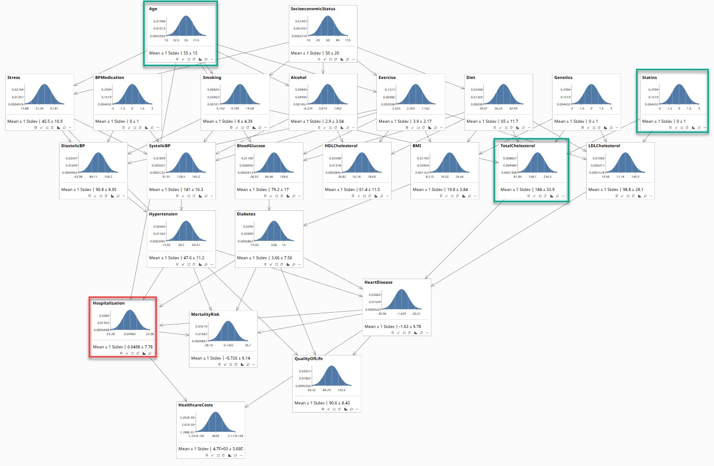
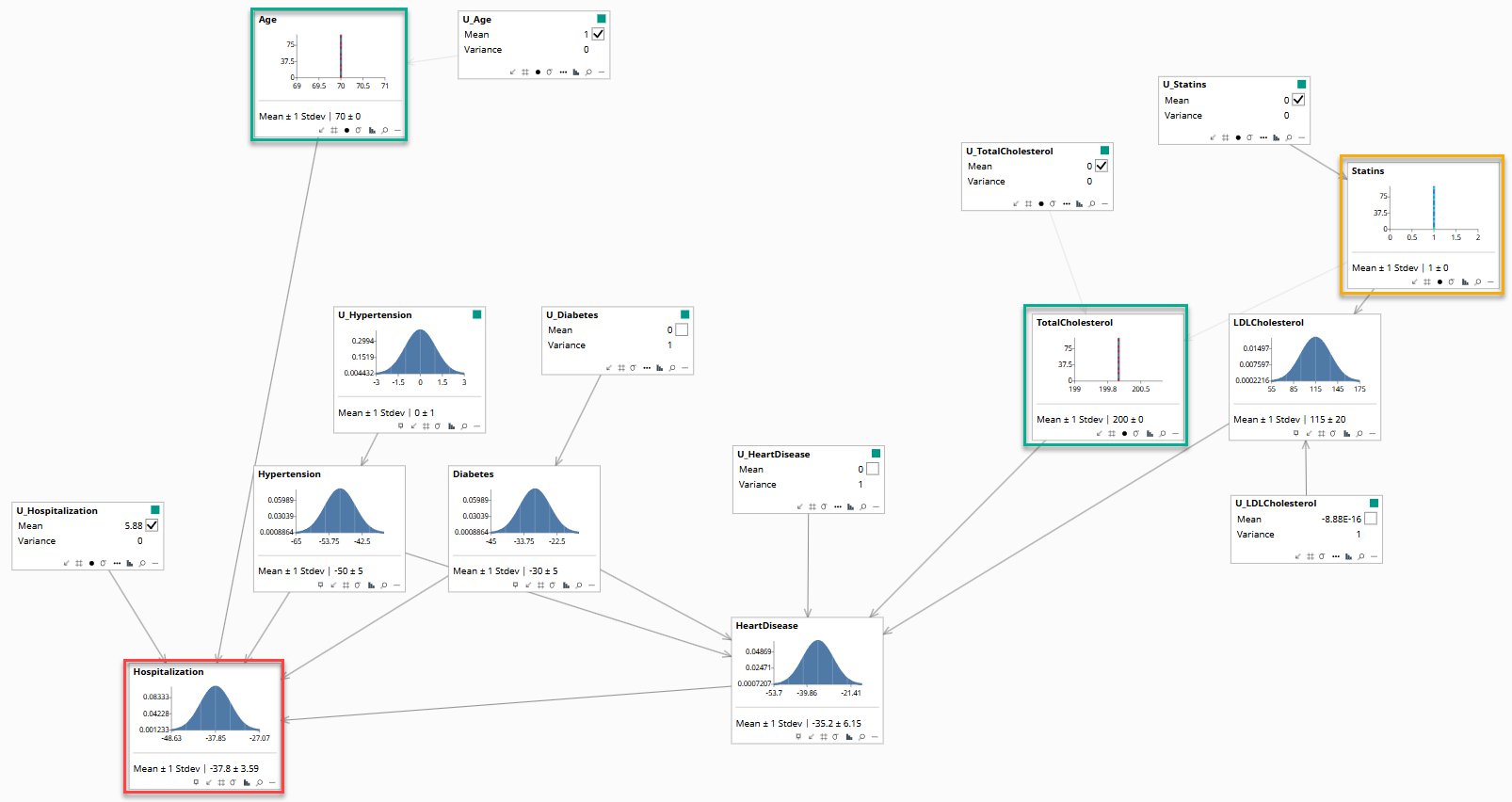
Each node is a variable your team agreed matters. Each arrow is a causal claim. The bell curves reflect population-level uncertainty. Green borders mark evidence nodes (Age, TotalCholesterol, Statins). Red border marks the query node (Hospitalization).
Either way the result is the same: causal claims your organization has committed to, in a form that can answer questions no dashboard can touch. The prompts shown below each diagram are shorthand instructions for producing each step.
The Causal Model
Build & Extend the Model
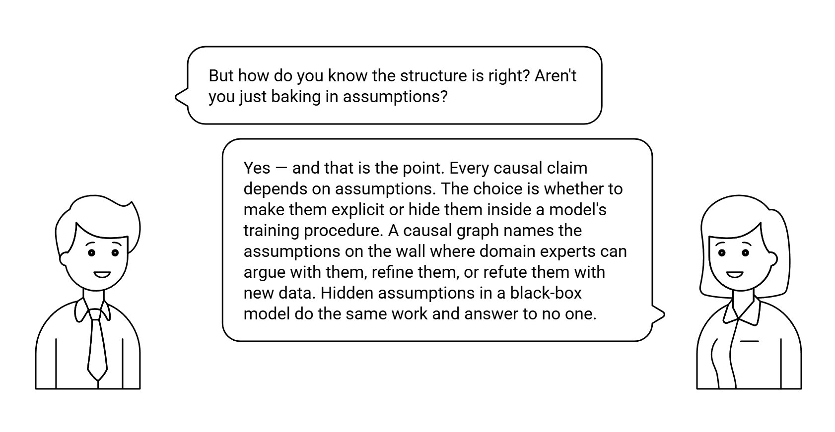
2. Extend to a Structured Causal Model
A U variable has been added beside each variable — representing everything that influences an outcome but is not in the data: genetics, lifestyle, unmeasured comorbidities. This is also the minimum causal subset of the full model. Right now the U variables are at their defaults. In the next step, the patient's observed data will allow the model to infer what these hidden factors must have been.
The Minimal Structured Causal Model
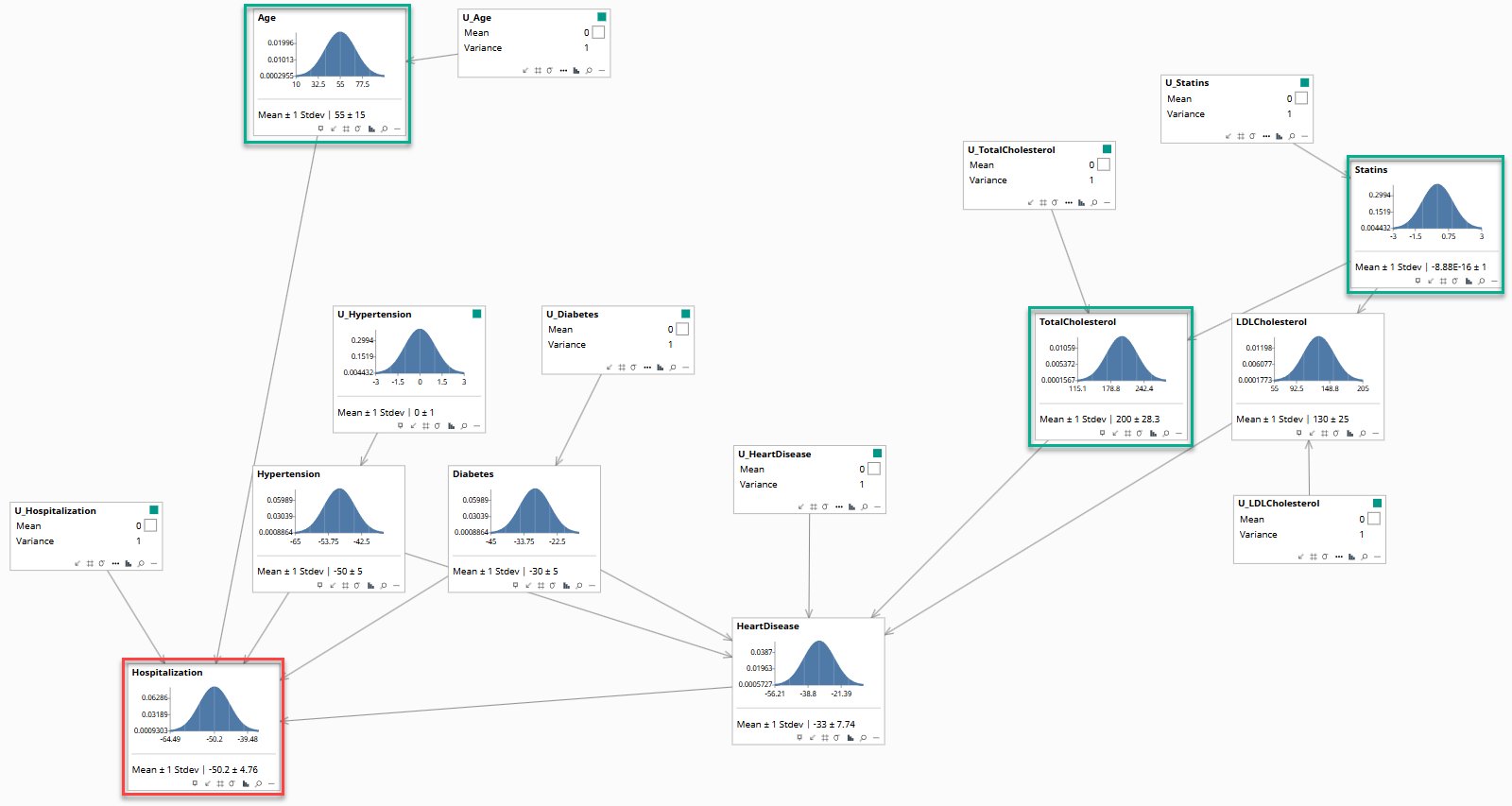
3. Answer the Counterfactual — what would have happened had statins been prescribed?
Abduction has been run. The model has inferred this patient's background factors. The broad curves have collapsed to narrow spikes. Statins (orange border) is fixed at zero: not prescribed. This is the factual world as it occurred.
After abduction, the model no longer represents the population. It represents this individual.
Abduction
Now the counterfactual question is asked: what would have happened if statins had been prescribed? The model applies do(Statins=1) — Pearl's notation for a direct intervention that sets a variable to a value, bypassing its normal causes — a supposition, not what actually happened. All hidden factors remain fixed at this patient's inferred values. Hospitalization shifts to −37.8 ± 3.59. That shift is the individual treatment effect. No heatmap, regression, or statistical model can produce this.
do(Statins=1)
Reading the Results
The observed fact is that this patient was hospitalised — Hospitalization = 1. After abduction, the model's continuous score reads −36.9 ± 3.59. The counterfactual, with statins prescribed, reads −37.8 ± 3.59. The two are almost identical.
That near-identity is not a flaw. It is an answer. The model is telling you that for this patient, the statin decision was not the primary driver of hospitalisation. The causal pathway from Statins runs through LDLCholesterol and then HeartDisease before reaching Hospitalization — three nodes, each attenuating the effect.
The reason the score sits at −36.9 rather than near 1 — despite the observed hospitalisation — lies in the U variable. After abduction, U_Hospitalization is inferred at 5.88. That large background factor reconciles the patient's observed outcome with everything else in the model. It represents unmeasured individual circumstances. That factor is held fixed in the counterfactual.
A population statistic says statin users are hospitalised 23% less often. That is true across the population. This model says: for this patient, the treatment effect was small. Both statements are correct. Only one is useful for a decision about this individual.
In risk management, the same distinction matters every time a loss occurs. A population rate tells you how often controls work across a portfolio. An individual treatment effect tells you whether this control would have prevented this loss — given this specific environment, this attack vector, this set of circumstances. That is the question a board asks after an incident. It is the question a regulator asks when reviewing a decision. It is what "root cause analysis" is attempting and failing to answer when it produces a timeline rather than a causal estimate. A structured causal model produces the estimate.
The question your board asks after every significant loss is a counterfactual. Now you can answer it.
info@rung3.ai
From a blank sheet to a working model — the same procedure applied to a full domain walkthrough: a property insurance rate-change decision, traced from first elicitation session to queryable model.
1 For illustration only. · 2 DAG — Directed Acyclic Graph: nodes are variables, arrows are causal claims, absence of cycles ensures a consistent probability distribution. · 3 Abduction is inference of a hypothesis from data.