Every causal model on this site is already a diagnostic model. No second system needs to be built. The transformer reliability model that predicts failure probability given operating conditions is the same model that identifies the most probable root cause given a failure event. The diagnostic capability is a free consequence of building the causal model at all.
One Model, Two Directions
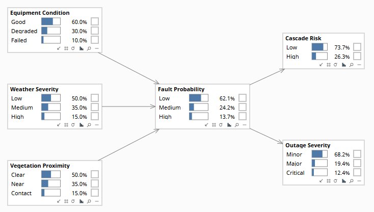
A Bayesian causal network encodes the conditional probability of each variable given its parents. The graph points from causes to effects: corrosion → insulation degradation → failure. The arrows represent the direction of causation.
The direction of inference is unrestricted. Bayes' theorem allows the network to be queried in either direction:
| Direction | Query | Interpretation | Use case |
|---|---|---|---|
| Forward | Set cause nodes; read effect node posteriors | Given what we know about conditions, what is the probability distribution over outcomes? | Prediction, risk assessment, simulation |
| Backward | Set effect node as evidence; read cause node posteriors | Given that this outcome occurred, what is the probability distribution over its causes? | Root cause analysis, diagnosis, attribution |
| Mixed | Set any combination of observed nodes; read posteriors on any unobserved nodes | Given everything observable, what is the probability distribution over everything unobserved? | Surveillance, anomaly explanation, decision support |
The mechanism that allows this is belief propagation — a message-passing algorithm that distributes the implications of new evidence through the entire network, updating every connected node's posterior probability. Evidence on any node propagates in all directions simultaneously: downstream toward effects, upstream toward causes, and laterally to nodes connected through common parents or common children.
A system built exclusively for prediction can be optimized for forward accuracy — AUC, calibration, discrimination. A Bayesian causal model built for decision-making is also a diagnostic model, a simulation engine, and an anomaly explanation system. The investment in building the causal graph and eliciting the conditional probability tables does not produce one capability. It produces five, on the same infrastructure. Diagnostic reasoning is one of them — and it comes at no additional cost once the graph exists.
Building a Prediction Model
Building a causal prediction model requires three of the five standard variable types: events (the conditions you are reasoning about), state (the system's vulnerability or configuration at the time of the event), and consequences (the outcomes the model is predicting). The causal order is Events → State → Consequences. The graph encodes which variables cause which. The conditional probability tables quantify how strongly.
What building it looks like
- Define the outcome variable. What is the model predicting? A failure event, a loss amount, a claim, a default. This is the downstream node the forward query will read.
- Identify the causal drivers. Which variables cause the outcome? Which cause each other? This produces the graph structure — the arrows drawn by domain experts.
- Populate the conditional probability tables. For each node, how probable is each value given the values of its causes? From data, from expert elicitation, or both.
- Validate forward. Does the model’s predicted distribution match historical outcomes? Calibration and discrimination tests apply here as they would to any probabilistic model.
What the prediction model produces
A probability distribution over the outcome variable — not a point estimate, but a full distribution that propagates uncertainty correctly through the causal chain. For every configuration of inputs, the model computes P(outcome | inputs). For any observed subset of inputs, it computes the marginal distribution over the outcome given the available evidence.
Sensitivity analysis is available without additional work: the model already knows which input variables most drive the output distribution. Importance factors (see Bayesian Risk Decisions) quantify this formally.
The diagnostic capability at no extra cost
A prediction model built correctly — with the causal graph explicit and the conditional probability tables populated — is already a diagnostic model. No second system needs to be built. The same graph that computes P(failure | conditions) also computes P(conditions | failure). The same parameters. The opposite inference direction.
This is not a design choice — it is a mathematical consequence of belief propagation. If the prediction model is correct, the diagnostic model is correct. If the graph is wrong, both are wrong in the same way — and the diagnostic queries will help find the error.
How Backward Inference Works
Transformer T-4471 tripped offline at 2:47 AM. The operations team must determine the root cause before committing to repair ($85K, three days) or replacement ($340K, six weeks). The transformer diagnostic model contains nine possible root causes, fourteen intermediate mechanisms, and twenty-two observable symptoms.
Enter the observed evidence
Set the observed symptom nodes to their observed values: Buchholz relay = Activated, Oil temperature = Elevated, External damage = None. These three observations are entered as hard evidence — the model now treats them as certain.
Propagate the evidence
Belief propagation distributes the implications of the three observations through the network. Every upstream node — every possible cause — has its posterior probability updated to reflect how consistent it is with all three observations simultaneously. Causes that would predict all three symptoms are pushed up. Causes that would predict one but not the others are pushed down.
Read the ranked posteriors
The model produces a ranked list of root causes by posterior probability, conditioned on all three observations:
| Root cause | Prior probability | Posterior (given 3 observations) |
|---|---|---|
| Insulation breakdown | 18% | 42% |
| Partial discharge | 15% | 22% |
| Overloading | 20% | 15% |
| Winding displacement | 12% | 9% |
| Bushing failure | 10% | 6% |
| All others | 25% | 6% |
Insulation breakdown is the most probable cause at 42% — more than double its prior — but 42% is not enough confidence to commit to an $85K repair over a $340K replacement. The model identifies the highest-VOI next test: dissolved gas analysis (DGA), which specifically discriminates between insulation breakdown and partial discharge.
DGA result: Hydrogen = High, Acetylene = High, Ethylene = Moderate. This pattern (high H2 + high C2H2) is characteristic of arcing in oil-impregnated insulation. Updated posteriors:
| Root cause | Posterior after DGA | Change |
|---|---|---|
| Insulation breakdown | 78% | +36pp |
| Partial discharge | 12% | −10pp |
| Overloading | 4% | −11pp |
| All others | 6% | −3pp |
78% confidence. Still not enough to distinguish localized (repairable) from widespread (replace) insulation damage. One more test: Frequency Response Analysis (FRA), VOI $24,500, cost $3,200. FRA result: normal response across all windings — no evidence of widespread deformation. Final posterior: localized insulation breakdown, 91%. Decision: repair. Total diagnostic cost: $5,000. Expected saving over blind replacement: $250,000.
Explaining away — when one cause changes the probability of another
A property of Bayesian networks that has no analog in classical diagnostic tools: confirming one cause automatically reduces the posterior probability of alternative causes, even when those alternatives are not directly tested. This is “explaining away” — the effect is explained by one hypothesis, which makes competing hypotheses less necessary.
In the transformer example: once the DGA confirms the pattern consistent with insulation breakdown, the probability of partial discharge falls from 22% to 12% — not because partial discharge was tested and ruled out, but because the evidence is better explained by insulation breakdown, and the two causes compete to explain the same symptom. Explaining away is how the model focuses diagnostic attention without requiring exhaustive testing of every hypothesis.
Building an Alert System
A causal alert system is built on the prediction model — the same graph, the same parameters. The difference is that observation nodes are monitored continuously, and backward inference runs whenever an anomaly is detected. Instead of: "Metric X exceeded threshold", the system produces: "Hypothesis A (posterior 67%): metric X is most probably driven by a shift in upstream variable Z. Hypotheses B and C account for the remaining 33%. The following test would discriminate between A and B at a cost of $X."
What building it requires beyond the prediction model:
- Identified observation nodes. Which variables can be measured in real time or near-real time? These are the evidence inputs.
- Defined upstream hypothesis nodes. Which upstream variables, if they shifted, would produce the observable anomalies? These are the targets for backward inference.
- A decision threshold for escalation. At what posterior probability does the leading hypothesis warrant investigation? Below what VOI is further testing not worth the cost?
What it produces versus threshold alerting
| Threshold alerting | Causal alert system |
|---|---|
| 200 alerts per day | 3–5 upstream hypotheses, ranked by posterior |
| “Metric exceeded limit” | “Most probably caused by X (67%), possibly Y (21%)” |
| Fixed checklist for all incidents | Adaptive investigation: next step chosen by VOI |
| Alert rate rises with data volume | Hypothesis count is bounded by the causal graph |
| Each alert is independent | 43 downstream anomalies traced to one upstream shift |
The structural benefit: the 200 threshold breaches in a monitoring dashboard are almost always downstream consequences of a small number of upstream shifts. Backward inference collapses many alerts to few explanations — and the explanations are the things that can actually be investigated and addressed.
Domain examples
| Domain | Observations | Upstream hypotheses |
|---|---|---|
| Insurance claims | Claim pattern, loss type, timing | Legitimate loss shift, fraud pattern, coverage mismatch |
| IT operations | Latency, error logs, service degradation | Network failure, deployment bug, capacity exhaustion |
| Manufacturing | Out-of-spec measurements, field returns | Material batch, machine calibration, operator error |
| Financial reporting | Unusual variance, ratio deviations | Market shift, accounting error, fraud, model failure |
Sequential Diagnosis and VOI
A fixed diagnostic protocol — a checklist that specifies the same test sequence regardless of symptoms — wastes money on tests that no longer discriminate between the remaining hypotheses. After the DGA result in the transformer example, running a power factor test (which discriminates between insulation and bushing problems) has near-zero VOI: bushing failure is already at 2% posterior. The model will not recommend it.
Adaptive sequential diagnosis works as follows:
Compute the current stopping criterion
Is the posterior confidence on any single cause high enough to commit to the corresponding action? If so, diagnosis terminates — the information already gathered is sufficient. If not, continue.
Compute the VOI for every remaining test
For each test not yet run, compute the expected improvement in the decision — the probability-weighted gain in expected utility from running the test, given the current posterior. A test that has a high probability of pushing the leading hypothesis above the decision threshold has high VOI. A test that would confirm a hypothesis already near-ruled-out has near-zero VOI.
Select and run the highest VOI/cost test
The next test is the one with the highest ratio of expected decision improvement to cost. Run it, enter the result as new evidence, and return to step 1.
| ✗ Fixed protocol | ✓ Adaptive sequential | |
|---|---|---|
| Test sequence | Same regardless of intermediate results | Adapts after each result — only tests that discriminate between remaining hypotheses are recommended |
| Stopping criterion | All tests in protocol completed | Posterior exceeds decision threshold, or VOI of all remaining tests is less than their cost |
| Typical test count (transformer) | 6–8 standard tests, $14K total | 2–3 targeted tests, $5K total |
| Diagnostic confidence | High (all tests run), but some redundant | Equivalent confidence — the adaptive sequence reaches the same conclusion via a shorter path |
| Over-investigation | Common — tests are run after conclusion is already clear | Impossible by design — model will not recommend a test whose VOI is less than its cost |
The stopping criterion — terminate when the VOI of every remaining test is less than its cost — is the same decision rule that governs any information-gathering under uncertainty. The model does not just diagnose the failure; it tells the team when they have enough information to act and when further investigation would cost more than it is worth. This is the discipline that prevents both under-investigation (acting at 42% confidence on a $340K decision) and over-investigation (running six more tests after 91% confidence has been reached).
What Changes When the Causal Model Is the Diagnostic Model
Root cause analysis becomes quantitative
The output is a ranked probability distribution over candidate causes, not a brainstormed list from a working group. The ranking reflects the actual evidential support for each hypothesis given everything observed. The most probable cause is the one most consistent with the full joint evidence set — not the one that senior engineers found most plausible in a meeting.
Test selection becomes adaptive
The next investigation step is determined by the model — whichever test has the highest VOI given the current posterior. The sequence is different for every incident because the evidence is different for every incident. Fixed protocols are replaced by adaptive strategies that converge on the same diagnostic confidence in fewer steps.
Diagnosis has a cost and a stopping criterion
The model computes when investigation should stop: when the posterior exceeds the decision threshold, or when the VOI of every remaining test is less than its cost. Investigation no longer continues until all standard tests are exhausted. It terminates when the answer is good enough to act on — and the model knows when that point has been reached.
Alerts collapse to explanations
Monitoring output shifts from many threshold breaches to few causal hypotheses. The 200 anomalous readings that would otherwise generate 200 tickets are instead traced to 3 upstream shifts. Each shift is a hypothesis with a posterior, a VOI, and an investigation plan. The monitoring system directs attention rather than overwhelming it.
Explaining away prevents wasted investigation
Confirming one cause automatically reduces the probability of alternatives, even without testing them directly. Once the DGA confirms insulation breakdown, testing for bushing failure becomes unnecessary — the model has already reduced it to 2%. The investigation focuses on the remaining uncertainty, not the full hypothesis space.
Every diagnosis updates the model
Each diagnosed incident is new evidence about the conditional probability relationships in the causal graph. The DGA pattern that updated the transformer model from 42% to 78% confidence is information about the likelihood function for insulation breakdown. Encoded as a model update, it makes the next similar diagnosis faster and more accurate. The causal model compounds: each investigation improves the model that conducts the next one.
Every causal model your organization builds for prediction and decision-making is already a diagnostic model. The question is whether you are using it in that direction — and whether your investigation costs reflect what that capability is worth.
info@rung3.ai
Pearl, J., 1988, Probabilistic Reasoning in Intelligent Systems, Morgan Kaufmann · Jensen, F.V. & Nielsen, T.D., 2007, Bayesian Networks and Decision Graphs (2nd ed.), Springer · Heckerman, D., Horvitz, E. & Nathwani, B., 1992, “Toward Normative Expert Systems,” Methods of Information in Medicine 31(2) · Cowell, R.G. et al., 1999, Probabilistic Networks and Expert Systems, Springer