Why a Causal Model
The registrational trial — KEYNOTE-024 for pembrolizumab in PD-L1 ≥50% NSCLC — established a population-level interventional answer: in patients who meet the inclusion criteria and are randomly assigned to immunotherapy versus chemotherapy, the immunotherapy arm has better survival. That is a Rung 2 claim about the trial population.
The patient on the tumor board today does not live in the trial population. Their PD-L1 is 35%. Their TMB is 8. Their ECOG is 1. Their comorbidity burden is moderate. The relevant quantity is a Conditional Average Treatment Effect — the expected difference in outcome under immunotherapy versus chemotherapy, conditional on this patient's specific covariate profile. That quantity is not what the trial reports. And it is not what observational data identifies, because the same biomarkers that drive prescribing decisions are the biomarkers that drive response.
A high-PD-L1 patient is more likely to receive immunotherapy and more likely to respond to it. In observational data, the marginal correlation between immunotherapy and survival overstates the causal effect, because the patients who got the drug were the patients most likely to do well regardless. The treatment is doing some work; the selection is doing the rest. Standard regression cannot tell you how the work is split.
The Causal Structure
The DAG below encodes the prescribing decision and its consequences. Four pre-treatment covariates — genomic profile, driver mutation, performance status, comorbidity burden — drive both the treatment decision and the survival outcome. That is the formal definition of confounding.
| Node | States | Role |
|---|---|---|
| GenomicProfile | Favourable_PDL1+TMB+MSI · Favourable_PDL1 · Favourable_TMB · Unfavourable | Composite biomarker — confounder |
| DriverMutation | EGFR/ALK+ · KRAS+ · Other · None | Drives targeted-therapy preference — confounder |
| PerformanceStatus | ECOG 0 · ECOG 1 · ECOG ≥2 | Strongest single survival predictor — confounder |
| ComorbidityBurden | Low · Moderate · High | Affects both treatment tolerability and survival — confounder |
| Treatment | Immunotherapy · Chemotherapy | The decision node |
| Survival_12mo | Alive · Deceased | Primary outcome |
| SevereToxicity_90d | Yes · No | Safety outcome — affects net benefit |
All four pre-treatment covariates have edges to Treatment (the prescribing rule) and to Survival_12mo (direct biological effect on outcome). Treatment has edges to both Survival_12mo and SevereToxicity_90d. PerformanceStatus and ComorbidityBurden additionally affect toxicity tolerance.
For Rung 3 capability, each observable node has a corresponding U-node — an exogenous noise variable that absorbs the residual variation not explained by the structural parents. These U-nodes are 50/50 priors that get abducted to a specific patient at counterfactual-evaluation time.
Under the back-door criterion, conditioning on {GenomicProfile, DriverMutation, PerformanceStatus, ComorbidityBurden} is sufficient to identify the interventional distribution P(Survival | do(Treatment)). What this does not address: physician gestalt, insurance status, patient preference — unmeasured factors that could create residual confounding. Sensitivity analysis (e-values, Rosenbaum bounds) quantifies how strong an unmeasured confounder would need to be to overturn the recommendation.
The Three Queries
The same DAG answers three operationally distinct questions. The graph does not change; only the query operator changes. Each panel below is a screenshot of the actual Bayes Server model — click a button to step through the slides.
How to read the diagrams. An arrow shows the causal direction. An arrow from A to B means A causes an effect — a change — in B.
Two operators appear repeatedly below. obs(X = value) means we learned that X had this value — like filtering the chart-review down to only patients where X was that value. do(X = value) means we imposed this value — like a randomization in a trial, where we control X regardless of what the patient would naturally have. The difference matters: filtering down to "patients who got the drug" tells you something about which patients tend to receive it; imposing the drug tells you only what the drug does.
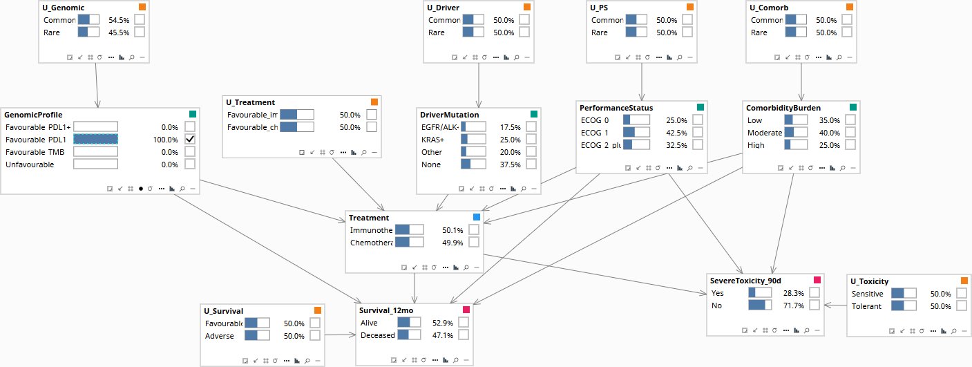
Among patients with this profile, what was the observed survival distribution?
Read directly from the data as a conditional probability. As more covariates are entered as evidence — GenomicProfile, PerformanceStatus, ComorbidityBurden — the survival number rises. But watch the Treatment node alongside: P(Immunotherapy) climbs even faster. The Survival_12mo improvement is partly biology, partly selection, and the conditional cannot tell you which is which.
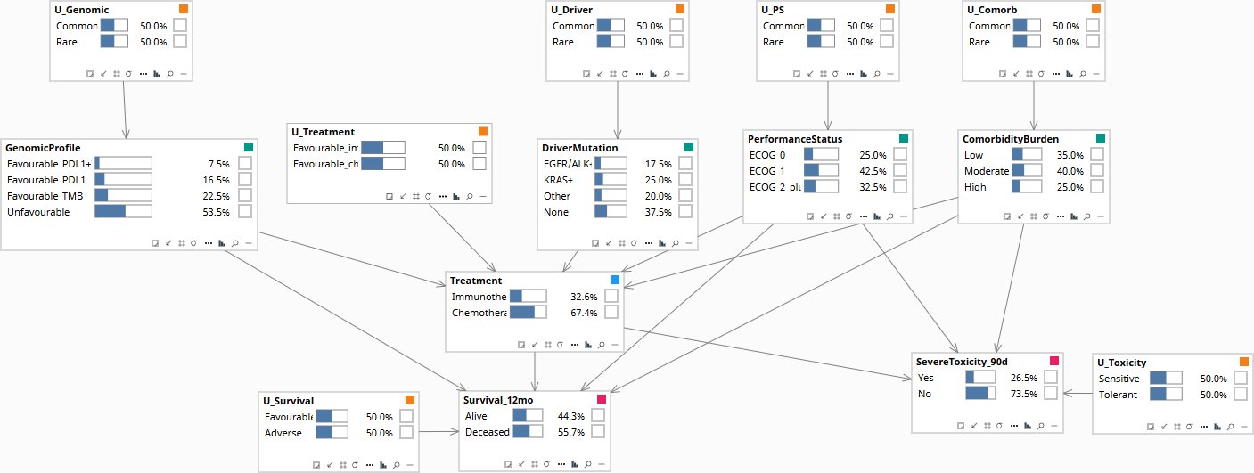
Population baseline before any patient data is entered. Survival, Treatment, and the covariates all sit at their marginal priors.
If we forced immunotherapy on a random patient — without conditioning on the prescribing rule — what would the survival distribution be?
The do-operator severs the incoming edges from GenomicProfile, DriverMutation, PerformanceStatus, and ComorbidityBurden into Treatment. What remains is the unconfounded population-level effect of the drug on Survival_12mo. Notice that the upstream covariates stay at their priors — the do-operator made the Treatment decision independent of them.
Population baseline. Treatment is at its prior — some patients on immunotherapy, most on chemotherapy, driven by natural prescribing.
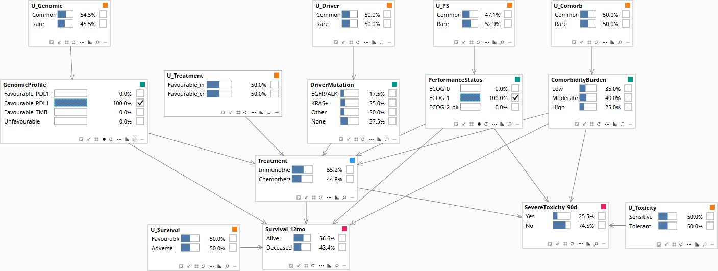
This specific patient received chemotherapy and survived 12 months. Would they have survived under immunotherapy?
Three operations on the same graph: (1) Set the patient's full evidence — GenomicProfile = Favourable_PDL1, PerformanceStatus = ECOG 1, ComorbidityBurden = Moderate, Treatment = Chemotherapy, Survival_12mo = Alive. The U_Survival posterior shifts away from 50/50 — that's the abduction step. (2) Carry the abducted U_Survival forward as soft evidence. (3) Apply do(Treatment = Immunotherapy) to read the counterfactual outcome.
Population baseline before any patient data is entered. All nodes at their marginal priors.
Download the Model
The Bayes Server file below encodes the DAG and the conditional probability tables described above. Each observable node has a corresponding U-node — the exogenous noise variable that absorbs residual variation — which is what makes Rung 3 counterfactual abduction possible. The CPTs are populated with clinically defensible illustrative priors; the qualitative behavior they encode is what makes the failure mode visible when running Rung 1 versus Rung 2 queries on the same data.